What Machines Actually Learn

The Weight of Intelligence Series — Part 1 A Socratic Guide to Machine Learning Fundamentals

The key to understanding AI: forget the metaphors. Look at the numbers.

Most explanations of machine learning start with neurons, layers, and analogies to the human brain. These metaphors feel intuitive, but they obscure what is actually happening underneath.

Open most modern ML models, from a spam filter to a code completion engine, and you will not find explicit rules or symbolic reasoning. You will find numbers. Millions of decimal values sitting in memory, waiting to be multiplied together. Those numbers are called weights and biases, and they are everything that training directly produces.

Understanding what weights are, how they are found, and why they sometimes fail is the key to understanding modern AI. That is what this series is about.

1. What do machines actually learn?

Let me be direct, because the terminology creates enormous confusion.

Training does not write concepts into a model as explicit rules. It does not store facts as retrievable entries or encode logic as if-then conditions. What training produces is parameters: a large set of numbers called weights and biases that shape how any input gets transformed into an output.

So where are the rules? There are none. Training only adjusts parameters.

Everything that looks like understanding, the convincing conversations, the apparently insightful code suggestions, the surprisingly correct answers, emerges from those parameters interacting with the model’s architecture. The parameters themselves are just numbers. Decimal numbers stored in computer memory, no different from the values sitting in a spreadsheet column.

This is not a subtle philosophical point. It is a practical engineering one. When a model fails, you stop asking “why did it decide that?” and start asking sharper questions: which parameters are miscalibrated, what data produced them, and what did we actually tell the training process to optimize for? Those questions have answers. “Why did it decide that?” usually does not.

But if parameters are just numbers, what makes one model smarter than another? That is where architecture comes in.

Architecture matters here too, but it is worth separating from parameters. Architecture is fixed before training begins. It determines the shape of the network: how many layers, how they connect, what operations they perform. Training’s job is to fill in the numbers. The architecture is the instrument. The parameters are the tuning.

2. What exactly is a weight?

In a simple model, a weight behaves like importance. That is the most useful starting intuition, and it holds up well enough to build on.

Here is an example almost everyone has lived through personally.

Imagine an airline wants to predict the total expected delay for a flight, from scheduled departure to actual arrival. They start simple, with one piece of data: the distance of the route in miles. Longer routes have more exposure to en-route weather, more complex logistics, and more opportunities for schedule compression to unravel. But they need a number, a way to turn distance into a delay estimate.

After studying a year of historical flights, they find a reasonable rule of thumb: roughly 0.04 minutes of expected delay per mile of route distance.

The model is now:

Predicted Delay (minutes) = Distance (miles) × 0.04

A 300-mile hop? About 12 minutes of expected delay. An 800-mile flight? Around 32 minutes. That number, 0.04, is a weight. It captures the learned relationship between one input signal and the predicted output.

Now notice something the model is ignoring. Even on a route with zero miles, before any flight-specific factor enters the picture, there is a floor of delay built into every departure: gate pushback time, taxi queue, standard turnaround. A typical airport adds around 8 minutes of baseline delay to almost every flight regardless of where it is going. That baseline, independent of any specific feature of the route, is what we call a bias in ML.

In the model, it looks like this:

Predicted Delay (minutes) = (Distance × 0.04) + bias

If the average baseline processing time across all departures is 8 minutes, the bias would be 8. Training learns this number the same way it learns the weight: by adjusting it until predictions better match reality across the data.

Real flight delays depend on far more than distance, of course. Weather, how busy the airport is, time of day, whether the inbound aircraft is running late. A fuller model has a weight for each signal:

Predicted Delay = (Distance × w₁) + (WeatherSeverity × w₂) + (AirportCongestion × w₃)
                + (TimeOfDay × w₄) + (InboundStatus × w₅) + ... + bias

Each weight tells the model how much to care about that input. A large positive weight means “this drives delays up.” A weight near zero means “this barely affects the estimate.” A negative weight would mean “this actually tends to reduce delays,” which might apply to a feature like whether the aircraft just completed maintenance.

One practical note: these features operate at very different scales. Distance might be in the hundreds of miles, WeatherSeverity might be a score from 0 to 10, and InboundStatus might be a simple 0 or 1 flag. In real models, you typically normalize features before training so that large-magnitude inputs do not dominate the parameter updates. It is a detail, but one that bites nearly every engineer the first time they extend a toy example to real data.

One important caveat before moving on. In this linear model, each weight has a fairly readable interpretation: importance. In deep neural networks, that clean interpretation breaks down. Individual weights are not interpretable on their own; what matters is how millions of them interact collectively to amplify or suppress patterns across many layers. The intuition, learned numbers shaping what gets emphasized or ignored, remains valid. The direct “weight equals importance” reading does not survive the jump to deep models.

If individual weights are not interpretable, how does the model mean anything at all? Meaning is distributed across many parameters and layers simultaneously. No single weight “stores” a concept any more than a single transistor “stores” a program.

When people say GPT-3 has 175 billion parameters, they mean a vast collection of learned weights and biases across many layers. (In practice, parameters also include embeddings and other learned scalars throughout the network. They are all the same thing: numbers found by training.) The architecture is far more complex than a single weighted sum. But the core principle is identical: a large set of numbers, found through training, determining how the model responds to any input.

3. What happens when the model is wrong?

Back to the flight delay model. A short 300-mile regional flight comes in. The model predicts 20 minutes of total delay (300 × 0.04 + 8 baseline bias = 20 minutes).

The flight arrives 3 hours late.

Why? The inbound aircraft had been diverted to an alternate airport the previous evening due to a runway closure there, and the repositioning added hours to its schedule. The model had no feature capturing inbound aircraft status. It looked at distance, saw a short easy hop, and produced a confident wrong answer.

In traditional programming, you would hunt for a logic error. You would read through conditional branches, find the broken assumption, and fix the code.

In machine learning, you do not fix logic. You fix numbers.

The model’s parameters were not miscalibrated exactly; they were optimized for a world where inbound disruptions were not a signal. To fix it, you add that signal and let training find its weight. You might also discover the existing weights need adjusting once the new feature changes the data distribution the optimizer sees.

This is what training actually is: iteratively adjusting parameters until the model’s outputs better fit the data. There is no mysticism involved. But there is an important nuance worth naming now, because it trips up almost every engineer the first time through.

In practice, you rarely hand-edit parameters directly. What you actually change is the data you feed in, the features you include, the loss function you define, or the length of training. The optimization process then finds better parameter values automatically. When your model gets something wrong in production, the fix almost never starts with the weights themselves. It starts with everything that shaped what those weights became.

That said, the question of how training adjusts parameters in the right direction is still unanswered. To get there, you need a way to measure wrongness precisely.

4. How does the model know it is wrong?

Every ML system needs a scorecard: a single number that quantifies exactly how wrong the current parameters are across the full training set. This is called a cost function or a loss function. Think of it as a Wrongness Meter.

The goal of training is not to make the model intelligent. The goal is simpler and more mechanical than that: get the Wrongness Meter as close to zero as possible on the training data.

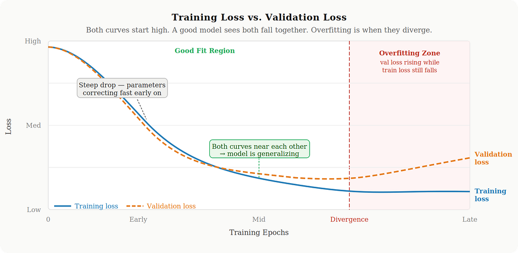
That last phrase matters. You minimize wrongness on training data, but you monitor wrongness on a separate validation set that the model never trained on. If training loss keeps dropping but validation loss stops improving or starts rising, you have overfit: the model has started memorizing the training examples rather than learning patterns that generalize. In practice, you always watch both curves.

5. The Wrongness Meter

The most common wrongness meter for regression problems is Mean Squared Error, or MSE:

Error = (Actual − Predicted)²

For the diverted aircraft scenario: the model predicted 20 minutes of total delay, actual was 180.

Error = (180 − 20)² = (160)² = 25,600

Across a full dataset of flights, you compute this for each one and average them. Training means finding parameters that make this average as small as possible.

For classification tasks and language models predicting the next token, the standard choice is cross-entropy loss rather than MSE. Cross-entropy measures how far the model’s predicted probability distribution is from the actual outcome. When you hear that an LLM was trained to “predict the next token,” cross-entropy is the loss behind that objective. MSE and cross-entropy feel different in their formulas, but they serve the same role: a single differentiable number that tells the optimizer which direction to move.

6. Why Squaring Matters

You might wonder why MSE squares the difference rather than just taking the absolute value. Two reasons, and understanding them reveals how the optimization process prioritizes its effort.

Reason one: errors cannot cancel each other out.

Suppose the model predicts 30 minutes of delay on two different flights:

• Monday: Predicted 30, Actual 40. Error: −10 (underpredicted by 10 minutes)
• Tuesday: Predicted 30, Actual 20. Error: +10 (overpredicted by 10 minutes)

Average raw error: (−10 + 10) / 2 = 0

The math would call this a perfect model. But the model was wrong on both flights, by 10 minutes each time. The errors cancelled. Squaring prevents this: Monday becomes 100, Tuesday becomes 100, average is 100. The loss correctly registers that predictions were off.

Reason two: large mistakes get penalized disproportionately.

• Miss by 5 minutes → penalty of 25
• Miss by 10 minutes → penalty of 100
• Miss by 50 minutes → penalty of 2,500
• Miss by 100 minutes → penalty of 10,000

Being off by 100 minutes is not 10 times worse than being off by 10. It is 100 times worse under MSE. This forces training to attack its biggest errors first. The optimizer will aggressively correct parameters that cause catastrophic misses, even if it means being slightly less accurate on easy cases.

That said, squaring makes MSE particularly sensitive to outliers. One extreme weather event that grounds flights for 6 hours can dominate the entire loss signal for that training batch. Mean Absolute Error, which skips the squaring step, handles those outliers more gracefully at the cost of a slightly noisier optimization signal. The choice of loss function is not a formality: it shapes what the model is actually trained to care about.

7. What training actually looks like

Now let us put all of this together with a concrete run.

Imagine you have a year of historical departure data: a sample of flights with their route distances and actual delay times. You want to find the best weight and bias automatically, without guessing.

Step 1: Start with random parameters.

You initialize the weight at some small arbitrary value, say 0.5, and the bias at 0.

Predicted Delay = (Distance / 1000) × 0.5 + 0

Dividing distance by 1000 keeps the input in the 0.1 to 1.2 range rather than the hundreds, which means the weight and bias learn at comparable speeds. Without this normalization, the large distance values produce gradient updates that overwhelm the bias, leaving it chronically undertrained. On a 300-mile flight with this starting point, the model predicts 0.15 minutes of delay. Almost certainly wrong.

Step 2: Measure total wrongness.

Run all flights in your dataset through the model. Compute squared error for each one, then average. Starting from 0.5, this score will be very high.

Step 3: Nudge the parameters in the right direction.

The training algorithm calculates which direction reduces error, and by how much. The mathematical technique behind this step is called gradient descent, and it is the subject of Part 2. For now it is enough to know that the algorithm has a precise, deterministic answer to “should this parameter go up or down, and by approximately how much?”

Weight and bias both get updated.

Step 4: Repeat.

Recalculate wrongness with updated parameters. It drops. Keep nudging. After many iterations, the wrongness stops decreasing meaningfully. Moving either parameter in any direction makes things worse. You have found the best values the algorithm can reach.

Step 5: Deploy.

When a new flight is scheduled, divide the route distance by 1000, multiply by the learned weight, add the learned bias, and return the delay estimate.

Here is what this loop looks like in Python:

# Flight data: (route_distance_miles, actual_delay_minutes)
raw_data = [
    (300, 20), (800, 40), (500, 28), (1200, 56), (200, 16),
    (400, 24), (1000, 48), (150, 14), (600, 32), (350, 22),
]

# Normalize distance so weight and bias gradients stay at comparable scales
training_data = [(d / 1000, actual) for d, actual in raw_data]
weight = 0.5   # random starting point
bias = 0.0
learning_rate = 0.01  # works stably with normalized input; Part 2 covers how to set this
for epoch in range(10000):
    for distance_k, actual in training_data:
        predicted = distance_k * weight + bias
        # Stochastic Gradient Descent: update parameters per example
        # Gradient of MSE with respect to weight and bias
        # Part 2 derives where these formulas come from
        weight_gradient = -2 * distance_k * (actual - predicted)
        bias_gradient   = -2 * (actual - predicted)
        weight -= learning_rate * weight_gradient
        bias   -= learning_rate * bias_gradient
print(f"Learned weight: {weight:.2f}")   # converges near 40 (minutes of delay per 1000 miles)
print(f"Learned bias:   {bias:.2f}")     # converges near 8 (baseline delay in minutes)

To translate the learned weight back into plain terms: a weight of 40 on normalized distance means 40 / 1000 = 0.04 minutes per mile, which is exactly the rule of thumb introduced in Section 2. The bias of roughly 8 matches the baseline gate and taxi delay described there too. The model started from random numbers and recovered both figures entirely on its own.

If you plotted the wrongness score over training, you would see a steep drop in the early epochs, then a long slow taper as the parameters close in on their best values. That shape, dramatic early progress followed by diminishing returns, is one of the most reliable patterns in ML training.

8. How does this scale to large language models?

Exactly the same way.

Start with random parameters (hundreds of billions of them). Feed in training data (an enormous corpus of text). Measure wrongness using cross-entropy: how badly did the model predict the next token in each sequence? Nudge parameters to reduce that wrongness. Repeat for weeks on large clusters of specialized hardware. Stop when the loss plateaus.

GPT-3’s 175 billion parameters were found through precisely this process. When you send a message to a language model, you are not talking to something that reasoned its way to knowledge. You are interacting with the output of a massive numerical optimization run. The model multiplies your input through 175 billion tuned parameters to produce output probabilities, which get decoded into tokens, which become the text you read.

Those parameters have captured real patterns: that questions tend to get followed by answers, that certain words appear near others in predictable ways, that code looks structurally different from prose. But the model did not learn those patterns the way you learn things. It found parameter values that minimized cross-entropy on a massive training corpus. What looks like understanding is an emergent property of having very well-tuned parameters at very large scale.

One honest clarification: modern transformer architectures involve attention mechanisms, layer normalizations, residual connections, and many stacked operations. They are considerably more complex than a single weighted sum. But every one of those operations ultimately resolves to arithmetic on learned parameters. The conceptual core holds all the way up: find numbers that minimize wrongness on the training objective. Same principle, vastly more parameters, vastly more data, vastly more compute.

When the model breaks, think this way

Once you see ML as a process of finding parameters that minimize a loss function, your instincts for debugging change.

When a model fails in production, the useful questions are:

Are we seeing distribution shift? The parameters were optimized for data that looked a certain way. A delay model trained entirely on summer schedules will underperform badly during winter storm season. If production inputs look meaningfully different from training data, expect the model to struggle. This is one of the most common and underappreciated failure modes in deployed systems.

Did we measure the wrong thing? The loss function defines what “good” means during training. If you optimized for the wrong objective, whether because of a poor proxy metric or evaluation leakage between training and validation, the model learned to be good at the wrong thing. The parameters will be exactly right for an objective you do not actually want.

Did training stop too early? Parameters that have not fully converged will leave predictable error on the table. Learning curves tell this story clearly.

Was the model too small for the problem? No amount of training corrects for insufficient capacity. A model with too few parameters cannot represent the patterns in the data regardless of how long you train it.

When a model succeeds, the same framing pays off. What was in the training data? What loss function did the team choose, and why? Did they watch validation carefully? Those choices shaped the parameters, and the parameters shaped everything you are seeing.

What is next

Training is finding parameters that minimize a loss function. But we have deferred the most important question in the entire field.

How does the algorithm know which direction to nudge?

With a single weight, you could try both directions by hand. With 175 billion parameters, trying every combination would take longer than the age of the universe. There must be a smarter approach, and there is.

The answer involves something that looks like navigating a foggy mountain in the dark, using nothing but the slope beneath your feet to decide your next step. It turns out to be one of the most elegant ideas in applied mathematics, and it is the engine behind every AI system you have ever used.

That is Part 2.

Summary

What do machines learn? Parameters: weights that scale input signals and biases that set baseline offsets.

How do they learn? By adjusting those parameters until predictions match reality across a training dataset.

What guides the adjustment? A loss function, a Wrongness Meter, that collapses all prediction errors into a single number. MSE for regression. Cross-entropy for classification and language modeling.

What is the actual goal? Minimize that number on training data, while monitoring validation data to catch overfitting.

The next time someone says an AI “understands” something, remember: it found parameters that produce low loss on a training objective. Understanding is a human concept. Parameters are a mathematical one.

Part 1 of 3

Next: How Machines Actually Improve, covering loss landscapes, gradient descent, and the geometry of learning that makes every AI breakthrough possible.

What Machines Actually Learn was originally published in Level Up Coding on Medium, where people are continuing the conversation by highlighting and responding to this story.