Strip Away the Cloud, the API Keys, and the Internet Connection. What You Have Left Is Still a Fully Working Music Discovery System.
There is a specific frustration I keep running into with in-car infotainment systems. You are on the highway, both hands on the wheel, and you want to hear something with that particular feeling, not a playlist name, not a genre label, but a vibe you cannot quite describe in three words. The car’s system gives you a search bar. You are expected to type. On a touchscreen. At 80 km/h.
The irony is that the technology to solve this has existed for years. Semantic search, voice transcription, vector embeddings. What has been missing is someone putting it together in a way that actually runs on the device, without shipping your voice to a datacenter and waiting for a round-trip.
This is the blog about how I built that system. It is called CarTune.
The full source code is available on GitHub at the project repository. Everything in this article maps directly to files in that repo, and I will reference the exact file location for every code snippet.
What CarTune Actually Does
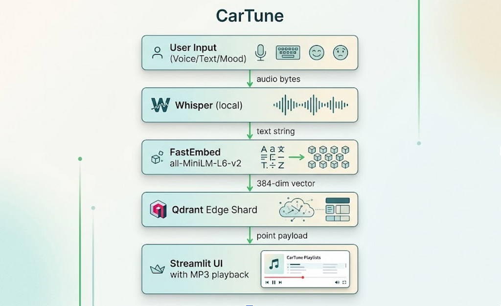
Before the architecture, let’s talk about the product. CarTune is a Streamlit application that runs entirely on-device. It does three things:
Voice search. The driver taps a button, speaks a request like “calm folk acoustic guitar,” and Whisper transcribes it locally. No speech-to-text API. No cloud call.
Text search. Natural-language queries like “upbeat hip hop for a long drive” get embedded into a 384-dimensional vector and searched against a local index of 7,994 songs.
Mood search. Six mood buttons (happy, sad, energetic, chill, romantic, party) expand into richer semantic queries and run the same vector search pipeline.
Every component runs on the same machine. The embedding model, the vector database, the transcription model, and the audio files all live on disk. The system works in airplane mode.
The Technology Stack at a Glance
The stack is deliberately minimal. Every dependency earns its place:
qdrant-edge-py — An embedded, in-process vector database. No server process. The index lives as a portable shard directory on disk.
fastembed — ONNX-based text embedding. Runs the all-MiniLM-L6-v2 model entirely on CPU. No GPU required, which matters for automotive hardware.
openai-whisper — Local speech transcription. The small model balances speed and accuracy well for voice queries.
mutagen — ID3 tag extraction from MP3 files. Used to build the metadata dataset from the Free Music Archive audio collection.
streamlit — The UI layer. Dark-themed, Spotify-inspired, with a custom HTML5 audio player that streams MP3 bytes from disk.
All of this is captured in pyproject.toml at the project root, with Python 3.10 to 3.12 support.
Step 1: Building the Dataset From Raw MP3s
The Free Music Archive (FMA) dataset ships as 8,000 royalty-free MP3 files organized in numbered subdirectories. There is no metadata CSV included. Every piece of useful information, track name, artist, album, genre, is embedded in the ID3 tags of each file.
The first pipeline step (scripts/prepare_dataset.py) walks the directory tree, reads those tags, and builds a unified data/songs.csv. Here is the core extraction function:
# scripts/prepare_dataset.py

def extract_track_metadata(filepath: Path) -> dict | None:
    """
    Read ID3 tags + audio info from a single MP3 file.
    Returns a dict ready for the songs.csv row, or None if the file is
    corrupt or has no usable title.
    """
    try:
        try:
            tags = ID3(filepath)
        except ID3NoHeaderError:
            tags = {}

        audio = MP3(filepath)
    except Exception as e:
        print(f"  [skip] {filepath.name}: {e}")
        return None

    title  = _safe_str(tags.get("TIT2"))
    artist = _safe_str(tags.get("TPE1"), "Unknown Artist")
    album  = _safe_str(tags.get("TALB"), "Unknown Album")
    genre  = _safe_str(tags.get("TCON"), "Unknown")

    duration_ms = int(audio.info.length * 1000) if audio.info.length else 0
    if duration_ms < 5000:    # under 5 seconds = corrupt
        return None

    moods = _genre_to_mood_defaults(genre)

    return {
        "track_id":         track_id,
        "track_name":       title,
        "track_artist":     artist,
        "track_album_name": album,
        "genre":            genre,
        "duration_ms":      duration_ms,
        "energy":           moods["energy"],
        "valence":          moods["valence"],
        "danceability":     moods["danceability"],
        "tempo":            moods["tempo"],
        "audio_path":       rel_audio_path,
    }
The _genre_to_mood_defaults() function is worth examining. Because FMA only provides genre tags (not the audio feature vectors you would get from Spotify’s API), this function maps genre strings to plausible energy, valence, danceability, and tempo values. The snippet below is an excerpt of the full function:
# scripts/prepare_dataset.py
def _genre_to_mood_defaults(genre: str) -> dict:
    g = genre.lower() if genre else ""

    presets = {
        "hip-hop":      (0.75, 0.55, 0.80, 95.0),
        "electronic":   (0.80, 0.55, 0.75, 125.0),
        "folk":         (0.35, 0.55, 0.40, 95.0),
        "ambient":      (0.20, 0.40, 0.25, 80.0),
        "punk":         (0.90, 0.55, 0.55, 150.0),
        "jazz":         (0.40, 0.55, 0.50, 110.0),
        # ... (energy, valence, danceability, tempo)
    }

    for key, vals in presets.items():
        if key in g:
            energy, valence, dance, tempo = vals
            return {
                "energy":       energy,
                "valence":      valence,
                "danceability": dance,
                "tempo":        tempo,
            }

    # neutral default
    return {"energy": 0.5, "valence": 0.5, "danceability": 0.5, "tempo": 120.0}
These are rough heuristics, not measured audio features, and the code is explicit about this. Folk music tends toward low energy and low danceability. Punk trends toward maximum energy. The values feed into the text descriptions that get embedded later, which is where they actually matter.
Running this script produces data/songs.csv with 7,994 usable rows. Each row carries the track metadata plus the relative path to its MP3 file on disk.
Step 2: The Embedding Pipeline
This is where the magic actually happens. The ingestion pipeline (src/ingest.py) reads the CSV, converts each song into a natural-language description, embeds those descriptions into 384-dimensional vectors, and stores everything in a Qdrant Edge shard.
Building Text Descriptions
The key insight is this: FastEmbed’s all-MiniLM-L6-v2 model works on text, not audio. So the first job is to translate each song’s metadata into a sentence that captures its character:
# src/ingest.py
def build_song_description(row):
    """
    Combine the most useful metadata fields into a single natural-language
    string. This is what we embed -- not the raw audio features.

    Example output:
        "Food by AWOL from the album AWOL - A Way Of Life. Genre: Hip-Hop.
         Mood: energetic, danceable."
    """
    name   = str(row.get("track_name", "")).strip()
    artist = str(row.get("track_artist", "")).strip()
    album  = str(row.get("track_album_name", "")).strip()
    genre  = str(row.get("genre", "")).strip()

    energy_val  = float(row.get("energy", 0.5) or 0.5)
    valence_val = float(row.get("valence", 0.5) or 0.5)
    dance_val   = float(row.get("danceability", 0.5) or 0.5)

    mood_words = []
    if energy_val > 0.7:
        mood_words.append("energetic")
    elif energy_val < 0.3:
        mood_words.append("calm")

    if valence_val > 0.7:
        mood_words.append("happy")
    elif valence_val < 0.3:
        mood_words.append("melancholic")

    if dance_val > 0.7:
        mood_words.append("danceable")

    mood_str = ", ".join(mood_words) if mood_words else "moderate tempo"

    description = (
        f"{name} by {artist} from the album {album}. "
        f"Genre: {genre_str}. "
        f"Mood: {mood_str}."
    )
    return description
This is a deliberate design choice. A text embedding model trained on natural language sentences understands the semantic relationship between words like “calm,” “acoustic,” and “folk” far better than it would understand a tuple of raw floats like (0.35, 0.55, 0.40, 95.0). Converting the numerical features back into language before embedding them closes this gap.
Generating Embeddings at Scale
# src/ingest.py

def generate_embeddings(descriptions, model_name=EMBEDDING_MODEL):
    print(f"[ingest] Initialising FastEmbed model: {model_name}")
    model = TextEmbedding(model_name=model_name)

    print(f"[ingest] Generating embeddings for {len(descriptions)} tracks ...")
    start = time.time()
    embeddings = list(model.embed(descriptions))
    elapsed = time.time() - start
    print(f"[ingest] Embedding done in {elapsed:.1f}s "
          f"({len(descriptions)/elapsed:.0f} tracks/sec)")

    return embeddings
The all-MiniLM-L6-v2 model runs at roughly 220 tracks per second on CPU via ONNX. Embedding all 7,994 songs takes about 36 seconds. This is a one-time cost. Once the shard is built, it stays on disk permanently and you never re-run this step unless the dataset changes.
The resulting vectors are 384 dimensions each, which means the raw vector data for the full dataset is approximately 7,994 × 384 × 4 bytes, around 11.7 MB. Qdrant Edge adds its HNSW index structure on top of this, but the total shard size remains well within the constraints of automotive storage hardware.
Step 3: Creating the Qdrant Edge Shard
Qdrant Edge is fundamentally different from Qdrant Cloud or a self-hosted Qdrant server. There is no server process to manage. You import qdrant_edge, point it at a directory path, and it handles the storage and indexing entirely in-process.
# src/ingest.py

def create_shard(shard_path=SHARD_DIR, dim=EMBEDDING_DIM):
    """
    Initialise a fresh Qdrant Edge shard on disk.
    Wipes any existing shard at the same path so re-runs always start clean.
    """
    if os.path.exists(shard_path):
        print(f"[ingest] Removing old shard at {shard_path}")
        shutil.rmtree(shard_path)

    os.makedirs(shard_path, exist_ok=True)

    config = EdgeConfig(
        vectors=EdgeVectorParams(size=dim, distance=Distance.Cosine),
    )
    shard = EdgeShard.create(str(shard_path), config)
    print(f"[ingest] Created new Qdrant Edge shard at {shard_path}")
    return shard
The distance metric choice is Cosine. This is correct for sentence embeddings. We care about the direction of two embedding vectors in 384-dimensional space, which indicates semantic similarity, not their magnitude, which would reflect sentence length or embedding scale artifacts.
Indexing Songs with Full Payload
The indexing step stores not just the vectors but the complete song metadata as a Qdrant payload:
# src/ingest.py

def index_songs(shard, df, embeddings, batch_size=500):
    total = len(df)
    print(f"[ingest] Indexing {total} songs into Qdrant Edge ...")

    for batch_start in range(0, total, batch_size):
        batch_end = min(batch_start + batch_size, total)
        points = []

        for idx in range(batch_start, batch_end):
            row = df.iloc[idx]
            vector = embeddings[idx].tolist() if hasattr(embeddings[idx], "tolist") else list(embeddings[idx])

            payload = {
                "track_id":          str(row["track_id"]),
                "track_name":        str(row["track_name"]),
                "track_artist":      str(row["track_artist"]),
                "track_album_name":  str(row.get("track_album_name", "")),
                "playlist_genre":    str(row.get("genre", "")),
                "energy":            float(row.get("energy", 0.5) or 0.5),
                "valence":           float(row.get("valence", 0.5) or 0.5),
                "danceability":      float(row.get("danceability", 0.5) or 0.5),
                "tempo":             float(row.get("tempo", 120.0) or 120.0),
                "duration_ms":       int(row.get("duration_ms", 0) or 0),
                "audio_path":        str(row.get("audio_path", "")),
            }

            points.append(Point(idx, vector, payload))

        shard.update(UpdateOperation.upsert_points(points))
        print(f"  ... indexed {batch_end}/{total} tracks")

    shard.flush()
The audio_path field in the payload is the key that connects the vector index back to the actual MP3 file on disk. When a user clicks Play, the player reads this path and loads the file bytes. This means the entire system, from search to playback, is self-contained without any network calls.
Step 4: Semantic Search at Query Time
The search module (src/search.py) handles the runtime query path. Both the embedding model and the shard are loaded lazily on first use and kept in memory as module-level singletons to avoid startup cost on every query:
# src/search.py

_embedding_model = None
_shard = None

def _get_model():
    """Lazy-load the FastEmbed model."""
    global _embedding_model
    if _embedding_model is None:
        print("[search] Loading FastEmbed model ...")
        _embedding_model = TextEmbedding(EMBEDDING_MODEL)
    return _embedding_model

def _get_shard():
    """Lazy-load the Qdrant Edge shard from disk."""
    global _shard
    if _shard is None:
        print(f"[search] Loading Qdrant Edge shard from {SHARD_DIR} ...")
        _shard = EdgeShard.load(str(SHARD_DIR))
        info = _shard.info()
        print(f"[search] Shard loaded -- {info.points_count} points indexed.")
    return _shard
The main search function embeds the query text and runs an approximate nearest-neighbor lookup:
# src/search.py

def search_songs(query_text, top_k=DEFAULT_TOP_K, genre_filter=None):
    shard = _get_shard()
    query_vector = embed_query(query_text)

    # Optional payload filter
    search_filter = None
    if genre_filter:
        search_filter = Filter(
            must=[
                FieldCondition(
                    key="playlist_genre",
                    match=MatchTextAny(text_any=genre_filter.lower()),
                )
            ]
        )

    request = SearchRequest(
        query=Query.Nearest(query_vector),
        filter=search_filter,
        limit=top_k,
        with_payload=True,
        with_vector=False,
    )

    results = shard.search(request)

    songs = []
    for hit in results:
        song = dict(hit.payload)
        song["score"] = hit.score
        song["point_id"] = hit.id
        songs.append(song)

    return songs
This is an approximate nearest-neighbor search using HNSW (Hierarchical Navigable Small Worlds). For 7,994 points in 384 dimensions, the HNSW index delivers sub-millisecond query times on CPU. The trade-off versus exact search is a small recall loss (typically 95% or higher recall at default HNSW settings), which is completely acceptable for music discovery.
The Mood Expansion Pattern
The mood search wrapper demonstrates a useful pattern: expanding short, ambiguous user signals into richer semantic queries before embedding:
# src/search.py

def search_by_mood(mood, top_k=DEFAULT_TOP_K):
    mood_map = {
        "happy":     "happy upbeat cheerful song",
        "sad":       "sad melancholic slow emotional song",
        "energetic": "high energy fast loud workout song",
        "chill":     "calm relaxing lo-fi ambient chill song",
        "romantic":  "romantic love ballad slow dance song",
        "party":     "party dance club banger high energy song",
    }

    expanded = mood_map.get(mood.lower(), mood)
    return search_songs(expanded, top_k=top_k)
A single word like “chill” carries limited semantic information for an embedding model. “Calm relaxing lo-fi ambient chill song” has far more dimensional coverage of the concept in embedding space, producing better recall across the songs indexed with descriptions like “calm, moderate tempo” or “ambient, instrumental.”
Step 5: Voice Transcription with Whisper
The voice pipeline (src/voice.py) is the most straightforward module in the codebase, which is a testament to how good Whisper’s API is:
# src/voice.py

_whisper_model = None

def _get_whisper():
    """Load the Whisper model once and keep it in memory."""
    global _whisper_model
    if _whisper_model is None:
        print(f"[voice] Loading Whisper model: {WHISPER_MODEL} ...")
        _whisper_model = whisper.load_model(WHISPER_MODEL)
        print("[voice] Whisper model loaded.")
    return _whisper_model


def transcribe_audio_file(audio_path):
    model = _get_whisper()
    result = model.transcribe(str(audio_path), language="en", fp16=False)
    text = result["text"].strip()
    print(f"[voice] Transcription: '{text}'")
    return text


def transcribe_uploaded_audio(audio_bytes, suffix=".wav"):
    """
    For the Streamlit UI: takes raw audio bytes from the audio input component,
    writes them to a temp file, and transcribes.
    """
    tmp = tempfile.NamedTemporaryFile(suffix=suffix, delete=False)
    tmp.write(audio_bytes)
    tmp.flush()

    text = transcribe_audio_file(tmp.name)
    return text
The fp16=False flag matters. Whisper defaults to half-precision on the GPU. On CPU-only hardware, you need full precision or the model will silently fail. This is the kind of footgun that sends engineers to Stack Overflow at 11 PM, so it is worth calling out explicitly.
The small model balances transcription quality with memory footprint. It handles accented English well enough for most voice queries, loads in a few seconds, and requires approximately 461 MB of disk space for the model checkpoint. Runtime RAM usage is in a similar range.
Step 6: The Music Player
The player module (src/player.py) is an intentionally simple state machine. Its job is to load MP3 bytes from disk and keep them in Streamlit’s session state so the audio element persists across reruns:
# src/player.py
def play(self, song_info: dict) -> bool:
    """
    Load the MP3 for the given song and mark it as playing.
    Returns True on success, False if the audio file is missing.
    """
    self.current_song  = song_info
    self.error_message = None

    rel_path = song_info.get("audio_path", "")
    candidate = Path(rel_path)
    if not candidate.is_absolute():
        candidate = PROJECT_ROOT / candidate

    if not candidate.exists():
        self.error_message = f"Audio file not found: {candidate}"
        self.is_playing = False
        return False

    try:
        with candidate.open("rb") as f:
            self.audio_bytes = f.read()
    except Exception as e:
        self.error_message = f"Failed to read audio file: {e}"
        self.is_playing = False
        return False

    self.audio_path = str(candidate)
    self.is_playing = True
    return True
The player handles both relative paths (stored in the shard payload as fma_small/000/000002.mp3) and absolute paths, which makes the system portable across machines without re-indexing.
The Custom HTML5 Audio Player
The standard Streamlit st.audio() component works, but it does not look or feel like anything you would want in a car dashboard. The custom audio player (src/audio_player.py) renders a Spotify-styled HTML5 player using embedded base64 audio and base64-encoded PNG icons:
# src/audio_player.py (excerpt)

def render_audio_player(audio_bytes, title, artist, album="", duration_str="0:30") -> str:
    b64_audio = base64.b64encode(audio_bytes).decode("ascii")

    # Load PNG icons as base64 data URIs for the embedded HTML
    play_src  = load_icon_b64_src("play-buttton.png")
    pause_src = load_icon_b64_src("video-pause-button.png")
    next_src  = load_icon_b64_src("play.png")

    return f"""
    <audio id="sp-audio" autoplay>
        <source src="data:audio/mpeg;base64,{b64_audio}" type="audio/mpeg" />
    </audio>
    <!-- Spotify-styled progress bar, play/pause button, volume control -->
    """
The entire MP3 file is base64-encoded and embedded as a data URI inside the HTML. This avoids the need for a local file server. The trade-off is that large files inflate the HTML payload significantly. For a 30-second audio sample, this is fine. For a full 4-minute track, the base64 string alone can be several megabytes embedded in the DOM, which is why there is a real-world case for streaming instead of targeting production deployment.
The Central Configuration File
Every path, model name, and default value lives in src/config.py. This is a small but important architectural decision:
# src/config.py

PROJECT_ROOT = Path(__file__).resolve().parent.parent

DATA_DIR  = PROJECT_ROOT / "data"
SHARD_DIR = DATA_DIR / "qdrant_shard"
SONGS_CSV = DATA_DIR / "songs.csv"
FMA_DIR   = PROJECT_ROOT / "fma_small"

EMBEDDING_MODEL = "sentence-transformers/all-MiniLM-L6-v2"
EMBEDDING_DIM   = 384
DISTANCE_METRIC = "Cosine"
WHISPER_MODEL   = "small"
DEFAULT_TOP_K   = 5
When you want to swap the embedding model for a higher-dimensional alternative or change the default result count, you change one line in one file. Every other module imports from here. This is not just clever engineering, it is the obvious right way to structure a system with multiple interdependent components.
Why Qdrant Edge Over Alternatives
The comparison that matters most for an edge deployment is not Qdrant Edge versus Qdrant Cloud. It is Qdrant Edge versus every other approach you might consider for on-device vector search.
SQLite with vector extension. sqlite-vec and sqlite-vss work, but HNSW performance at this scale is noticeably slower, and the ecosystem around them is thinner.
FAISS in-memory index. FAISS is fast and battle-tested. But it does not persist natively. You have to serialize and deserialize the index yourself. You also lose payload filtering, which is the feature that lets you combine vector similarity with metadata constraints in a single query.
ChromaDB. Chromadb runs embedded. It is great for RAG prototypes. For automotive deployment, Qdrant Edge’s smaller footprint and the portability of its shard format (copy the directory and the index works identically on any machine) are meaningful advantages.
Cloud vector databases (Pinecone, Weaviate Cloud, Qdrant Cloud). These require the internet. That disqualifies them immediately for an in-car system where connectivity is unreliable by definition.
The shard portability point is underappreciated. Once you build the shard on your development machine, you copy the data/qdrant_shard/ directory to the target device, and the index works identically without re-indexing. No re-embedding. No re-training. Just copy and run.
What the Full Pipeline Looks Like End to End
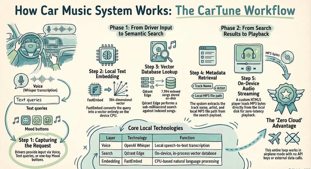
Here is the sequence from driver voice input to music playing, traced through the actual code:
- The driver taps the mic button in the Streamlit Voice tab (app.py — tab_voice section).
- Streamlit’s st.audio_input() captures the recording. Bytes are passed to transcribe_uploaded_audio() (src/voice.py).
- Whisper writes bytes to a temp file and transcribes. Returns a text string like “calm acoustic guitar.”
- The text goes to search_songs() (src/search.py).
- embed_query() encodes it with FastEmbed into a 384-dim vector.
- Qdrant Edge runs HNSW approximate nearest-neighbor search over 7,994 indexed vectors.
- Top-5 results come back with full payloads (track name, artist, audio_path).
- Results render as song cards in the left column.
- Driver taps Play on a result. MusicPlayer.play() (src/player.py) reads the MP3 from disk.
- render_audio_player() (src/audio_player.py) embeds the bytes as base64 in an HTML5 player.
- Streamlit renders the player. Audio plays in the browser without any network call.
Total latency from end of voice input to results displayed: the vector search itself completes in under a millisecond for 7,994 points. Whisper transcription dominates the total pipeline time. On a modern CPU, the small model processes a 3 to 5 second voice clip in roughly 5 to 20 seconds, depending on hardware. On ARM-based automotive chips, this is slower. GPU presence changes the calculation entirely. For a voice-first UI in a moving vehicle, this is the most significant engineering challenge in this architecture, and it is worth stress-testing on your target hardware before committing to Whisper small as the production choice.
Running the System Yourself
The setup is four commands after cloning the repo:
1. Install dependencies
uv venv && source .venv/bin/activate
uv pip install -r requirements.txt
2. Download FMA-small dataset
wget https://os.unil.cloud.switch.ch/fma/fma_small.zip
unzip fma_small.zip -d .
3. Build songs.csv from MP3 ID3 tags (one-off)
python scripts/prepare_dataset.py
4. Build the Qdrant Edge shard (one-off, ~36 seconds)
python -m src.ingest
5. Launch the app
streamlit run app.py
After step 4, the data/qdrant_shard/ directory persists. Future runs of streamlit run app.py skip directly to the search interface. The shard directory is excluded from git via .gitignore because at roughly 12 MB of vectors plus HNSW index overhead, it is appropriate to generate locally.
Limitations Worth Being Honest About
This is a working prototype with real production gaps, and pretending otherwise would not serve anyone who wants to build on it.
Audio features are genre-derived, not measured. The energy, valence, and danceability values come from _genre_to_mood_defaults(), a lookup table of heuristics. They are plausible approximations, not Spotify-quality acoustic analysis. A production system would use an audio feature extraction library like librosa or essentia to compute these from the actual audio signal.
Base64 audio embedding does not scale to full tracks. Encoding a full 4-minute MP3 as base64 in an HTML string is not ideal. A real deployment would serve the audio through a local HTTP server (a few lines of Python) and reference it by URL in the audio element, rather than embedding the entire file in the DOM.
Single-node, no persistence across sessions. Qdrant Edge creates a shard per process. If you want a multi-session state (user history, favorites, play counts), you need a lightweight persistence layer on top. SQLite works well for this.
Whisper small occasionally mispronounces artist names. Proper nouns are harder for the model. If “Fleetwood Mac” comes out as “Fleet with Mac,” the downstream search still works reasonably well because the embedding model handles near-misses in common English, but accuracy on niche artist names drops.
What This Pattern Enables Beyond Music
The architecture here is not specific to music. The same pipeline, local embeddings, an on-device Qdrant Edge shard, and a payload-enriched index works for any domain where you need semantic search without a cloud dependency:
Vehicle documentation retrieval. Index the car’s manual and service procedures. “Why is the tire pressure light on?” returns the relevant diagnostic section.
Offline enterprise knowledge bases. Field technicians with unreliable connectivity could search internal documentation, wiring diagrams, and parts catalogs through natural language queries.
Privacy-first personal document search. Notes, receipts, medical records. Nothing leaves the device.
The tooling has reached the point where this kind of system takes a week to build, not a month. The components (FastEmbed, Qdrant Edge, Whisper) are all production-quality, well-maintained, and genuinely designed to run in constrained environments.
Closing Thoughts
Ultimately, what I gained from building CarTune was a massive shift in my own perspective as a developer. It proved to me that “offline-first” AI is no longer a frustrating limitation, it’s a highly accessible feature. I no longer feel tied to cloud APIs or complex infrastructure to build smart, semantic applications. The barrier to entry has vanished.
This project gave me the confidence to pull AI out of the cloud and run it right where the user is, without sacrificing performance. Looking forward, I’m excited to push this architecture further: my next goal is to deploy this stack onto actual edge hardware like a Raspberry Pi to test it in a real car environment, and eventually bake in a lightweight local LLM for even richer, context-aware media recommendations.
If this guide helped you automate a tedious task today, there’s more where that came from. Follow Sarvesh Talele here on Medium for practical, step-by-step AI guides that actually make a difference in your workflow.
Sources and References
- Github Link: https://github.com/sarveshtalele/How-I-Built-a-Smart-In-Car-Media-Discovery-System
- Qdrant Edge Documentation — https://qdrant.tech/documentation/edge/
- FastEmbed Documentation (Qdrant) — https://qdrant.github.io/fastembed/
- OpenAI Whisper (GitHub) — https://github.com/openai/whisper
- Free Music Archive Dataset — https://github.com/mdeff/fma (Defferrard et al., ISMIR 2017)
- all-MiniLM-L6-v2 Model Card — https://huggingface.co/sentence-transformers/all-MiniLM-L6-v2
- HNSW Algorithm — Malkov & Yashunin, “Efficient and Robust Approximate Nearest Neighbor Search Using Hierarchical Navigable Small World Graphs,” IEEE TPAMI 2020
- Streamlit Documentation — https://docs.streamlit.io
- mutagen Documentation — https://mutagen.readthedocs.io/en/latest/
- CarTune GitHub Repository — Full source code available at the project’s GitHub page: https://github.com/sarveshtalele/How-I-Built-a-Smart-In-Car-Media-Discovery-System
How I Built a Smart In-Car Media Discovery System was originally published in Level Up Coding on Medium, where people are continuing the conversation by highlighting and responding to this story.