What is Walk-Forward Backtesting? Implementation in Python

Learn the foundations and implementation of a realistic backtesting pipeline

Backtests often look far better on paper than they do in live markets. The usual reason is not that the idea was completely wrong. It is that the strategy was tuned too closely to the past, then judged on the same data it was trained on.

That is exactly the problem we will address in this guide.

We are going to build a complete walk-forward backtesting pipeline in Python using AAPL data from 2010 onward. The pipeline will cover data retrieval using FMP APIs, a simple SMA crossover strategy, parameter optimisation, and a full walk-forward framework that repeatedly retrains the strategy on rolling historical windows and tests it on unseen data.

The goal here is not just to run a backtest. It is to understand how walk-forward optimisation works, why traders use it, and how to build a pipeline that evaluates a strategy on data it has not already been tuned on.

What exactly is Walk-Forward Optimisation?

Why regular backtests can be misleading

A normal optimisation workflow usually looks something like this: take a long stretch of historical data, test many parameter combinations, pick the best one, and then judge the strategy based on how well it performed on that same period.

The problem is obvious once you slow down and think about it. If the strategy is allowed to search through the past until it finds the combination that worked best there, then the final result is not a clean test anymore. It is partly a reflection of how well the strategy adapted itself to that specific sample.

That does not always mean the strategy is useless. But it does mean the result can look much better than what you would get in actual trading.

What WFO changes

Walk-Forward Optimisation changes the question.

Instead of asking, “What is the best parameter set for this whole dataset?”, it asks, “If I were actually trading through time, and periodically retuning the strategy as new data came in, how would it have behaved?”

That is a much tougher test.

Rather than finding one fixed set of parameters and using it everywhere, WFO keeps moving forward through the timeline. At each stage, it uses the information available up to that point, selects the best parameters from that context, and then checks how those parameters behave on the next unseen segment of market data.

This repeated process makes the backtest feel much closer to how a strategy would be managed in the real world.

Why this is more realistic

Markets do not stay still. A parameter combination that works well in one period may stop working when volatility changes, trend strength weakens, or the market shifts into a different regime.

A static backtest hides that problem because it compresses everything into one big historical exercise. WFO forces the strategy to keep proving itself over time.

That is why WFO often produces weaker numbers than a fully optimised backtest. But weaker does not mean worse. In many cases, it just means more honest.

A strategy that delivers modest results across many unseen periods is usually more credible than one that looks incredible on a single fully optimised historical run.

What this article is trying to show

The point of this guide is not to present WFO as a magic fix. It will not suddenly make a weak strategy robust.

What it does offer is a more realistic evaluation framework. It helps us separate strategies that only looked good in hindsight from those that can hold up better when the market moves forward and conditions change.

By the time we finish the implementation, that difference will be much easier to see in practice.

The workflow we’ll build

• Pull historical AAPL price data using FMP’s Historical EOD API
• Build a simple SMA crossover strategy with parameterised short and long windows
• Calculate key performance metrics such as total return, Sharpe ratio, and maximum drawdown
• Run a static optimisation over multiple SMA combinations
• Test those “best” parameters on a later unseen period to show why static optimisation can fail
• Implement a walk-forward optimisation loop that keeps re-evaluating the strategy through time
• Combine the out-of-sample results into a single performance series
• Compare different walk-forward setups by changing the training depth and re-optimisation frequency

Data Extraction

First, we should import the necessary modules and retrieve the prices. We will use FMP’s Historical Index Full Chart API to get the Apple stock prices from 2010. This should give us enough space to explain walk-forward backtesting.

import pandas as pd
import numpy as np
from datetime import datetime, timedelta
import requests
from itertools import product
import matplotlib.pyplot as plt

token = 'YOUR FMP TOKEN'

def get_prices(symbol: str, from_date: str) -> pd.DataFrame:
    url = f"https://financialmodelingprep.com/stable/historical-price-eod/full"
    params = {"apikey":token, "symbol":symbol, "from":from_date}
    resp = requests.get(url, params=params)
    df = pd.DataFrame(resp.json())
    df['date'] = pd.to_datetime(df['date'])
    df.sort_values(by='date', inplace=True)
    df.set_index('date', inplace=True)
    df = df[['open', 'low','high','close']]
    
    return df

prices = get_prices("AAPL", "2010-01-01")
prices.to_csv("AAPL_prices.csv")
prices = pd.read_csv("AAPL_prices.csv", index_col='date')
prices

Note: Replace <YOUR FMP TOKEN> with your actual FMP API key. If you don’t have one, you can obtain it by opening an FMP developer account.

Building the Strategy

We will implement a straightforward strategy using a short and a long SMA. When the short SMA is above the long SMA, it indicates an uptrend in momentum, and when it is below, it suggests a downtrend. This approach relies on just two parameters: the periods for the short and long SMAs.

You will notice that we will aim to have all parameters defined in functions so that we can later run our walk-forward backtesting.

def run_strategy(df_prices: pd.DataFrame, short_window: int, long_window: int) -> pd.DataFrame:
    df = df_prices.copy()
    
    df['short_sma'] = df['close'].rolling(window=short_window).mean()
    df['long_sma'] = df['close'].rolling(window=long_window).mean()
    
    df['signal'] = np.where(df['short_sma'] > df['long_sma'], 1, -1)
    
    df['position'] = df['signal'].shift(1)
    
    df['market_returns'] = df['close'].pct_change()
    df['strategy_returns'] = df['position'] * df['market_returns']
    
    df = df.dropna()
    
    return df

prices = get_prices("AAPL", "2010-01-01")
returns_df = run_strategy(prices, short_window=50, long_window=200)

Another useful function is the one that calculates the metrics we will use to determine the best parameters overall. These metrics are the return, the Sharpe ratio, and the drawdown.

def calculate_metrics(df_returns: pd.DataFrame, returns_col: str = 'strategy_returns') -> dict:
    returns = df_returns[returns_col].dropna()
    
    if len(returns) == 0:
        return {'total_return': 0.0, 'sharpe_ratio': 0.0, 'max_drawdown': 0.0}
    
    total_return = (1 + returns).prod() - 1
    
    mean_return = returns.mean()
    std_return = returns.std()
    sharpe_ratio = mean_return / std_return * np.sqrt(252) if std_return > 0 else 0.0
    
    cumulative = (1 + returns).cumprod()
    running_max = cumulative.expanding().max()
    drawdown = (cumulative - running_max) / running_max
    max_drawdown = drawdown.min()
    
    return {
        'total_return': total_return,
        'sharpe_ratio': sharpe_ratio,
        'max_drawdown': max_drawdown
    }

metrics = calculate_metrics(returns_df)
print("Strategy Metrics:")
for key, value in metrics.items():
    print(f"  {key}: {value:.3f}" if isinstance(value, float) else f"  {key}: {value}")

bh_returns = returns_df['close'].pct_change().dropna()
bh_metrics = calculate_metrics(pd.DataFrame({'strategy_returns': bh_returns}))
print("\nBuy & Hold Metrics:")
for key, value in bh_metrics.items():
    print(f"  {key}: {value:.3f}")

You will notice that, for this time only, we are presenting the Buy and Hold strategy. This illustrates that it is not comparable to the BnH strategy. We are using it solely to demonstrate the WFO.

Now, this will return returns of approximately 240%, where the BnH is 2,150%!

Strategy Metrics:
  total_return: 2.347
  sharpe_ratio: 0.421
  max_drawdown: -0.709

Buy & Hold Metrics:
  total_return: 21.664
  sharpe_ratio: 0.863
  max_drawdown: -0.444

Static Optimisation

Now let’s see how we optimise a strategy. We will develop a function named optimize_strategy that we will re-use later on during our walk-forward.

def optimize_strategy(df_prices: pd.DataFrame, param_grid: dict, weights: dict) -> tuple:
    best_score = -np.inf
    best_params = None
    
    param_names = list(param_grid.keys())
    param_ranges = list(param_grid.values())
    param_combinations = list(product(*param_ranges))
    
    for params in param_combinations:
        param_dict = dict(zip(param_names, params))
        
        if param_dict['short_window'] >= param_dict['long_window']:
            continue
            
        df_returns = run_strategy(df_prices, **param_dict)
        metrics = calculate_metrics(df_returns)
        
        score = sum(weights[metric] * value for metric, value in metrics.items())
        
        if score > best_score:
            best_score = score
            best_params = param_dict.copy()
    
    return best_params, best_score

param_grid = {
    'short_window': range(10, 51, 5),
    'long_window': range(60, 201, 10)
}
weights = {
    'total_return': 0.5,
    'sharpe_ratio': 0.25,
    'max_drawdown': -0.25  
}

best_params, best_score = optimize_strategy(prices, param_grid, weights)
print(f"Best params: {best_params}")
print(f"Best score: {best_score:.4f}")

best_returns = run_strategy(prices, **best_params)
best_metrics = calculate_metrics(best_returns)
print("Best strategy metrics:", best_metrics)

Let’s break and understand the above code:

• The function will run all possible scenarios and return the best parameters that yield the optimal results
• We will calculate the “best result” based on the weights dictionary. Return will be weighted at 50% importance, the Sharpe Ratio at 25%, and the drawdown at 25%.
• Also, the range of parameters that we will run is defined in the param_grid. The short window will be from 10 to 50 with a step of 5, and the long from 60 to 200 with a step of 10.

When we run the code, we will get the results.

Best params: {'short_window': 40, 'long_window': 190}
Best score: 4.7696
Best strategy metrics: 
{
  'total_return': np.float64(8.9546466471214), 
  'sharpe_ratio': np.float64(0.6712458027118039), 
  'max_drawdown': np.float64(-0.4980050717114106)
}

The results indicate that the best strategy involves a short period of 40 (compared to 50 in the first run) and 190 (compared to 200). Interestingly, the parameters are very similar, yet the difference in results is substantial. It achieves an 895% return versus 240%, despite having slightly worse Sharpe ratio and drawdown.

Why Static Optimisation Fails

Now, let’s see what would have happened if we turned back the clock. Assuming that we are at the beginning of 2025, we will optimise the strategy using all available information up to the end of 2024, and run the results for the rest of the period.

prices_copy = prices.copy()
prices_copy.index = pd.to_datetime(prices_copy.index)

train_prices = prices_copy.loc[:'2024-12-31'].copy()
test_prices = prices_copy.loc['2025-01-01':].copy()

best_params_2024, best_score_2024 = optimize_strategy(train_prices, param_grid, weights)

warmup_needed = best_params_2024['long_window']
test_start_idx = prices_copy.index.get_loc(test_prices.index[0])
run_start_idx = max(0, test_start_idx - warmup_needed - 1)

test_with_warmup = prices_copy.iloc[run_start_idx:].copy()
post_2024_results = run_strategy(test_with_warmup, **best_params_2024)
post_2024_results = post_2024_results.loc[test_prices.index[0]:].copy()

post_2024_results['short_window'] = best_params_2024['short_window']
post_2024_results['long_window'] = best_params_2024['long_window']
post_2024_results['strategy_equity_curve'] = (1 + post_2024_results['strategy_returns']).cumprod()
post_2024_results['buy_hold_equity_curve'] = (1 + post_2024_results['market_returns'].fillna(0.0)).cumprod()

train_best_returns = run_strategy(train_prices, **best_params_2024)
train_best_metrics = calculate_metrics(train_best_returns)
post_2024_metrics = calculate_metrics(post_2024_results)
post_2024_bh_metrics = calculate_metrics(post_2024_results, 'market_returns')

print(f"Best params through 2024: {best_params_2024}")
print(f"Best score through 2024: {best_score_2024:.4f}")
print("Train metrics through 2024:", train_best_metrics)
print("Post-2024 strategy metrics:", post_2024_metrics)
print("Post-2024 buy & hold metrics:", post_2024_bh_metrics)

We will get the following results:

Best params through 2024: {'short_window': 40, 'long_window': 190}
Best score through 2024: 5.7777
Train metrics through 2024: {'total_return': np.float64(10.924030420948082), 'sharpe_ratio': np.float64(0.7648261444219087), 'max_drawdown': np.float64(-0.4980050717114106)}
Post-2024 strategy metrics: {'total_return': np.float64(-0.16516091491739893), 'sharpe_ratio': np.float64(-0.32810384163758666), 'max_drawdown': np.float64(-0.3552200321799349)}
Post-2024 buy & hold metrics: {'total_return': np.float64(0.028112770545483334), 'sharpe_ratio': np.float64(0.2310467501453109), 'max_drawdown': np.float64(-0.30222581950627286)}

So this means that the best parameters are 40 and 90 (as before), but guess what? If we used the those parameters for the rest of the period (2025 till today) we would have lost 16.5% of our invested capital!

Implementing Walk Forward Optimisation

So, now let us explain walk-forward optimisation. What is important at this point are the two basic parameters: the reoptimisation period and the training period. What does that mean?

The reoptimisation period refers to the timeframe in which we’ll update our strategy. In the example below, we will perform an initial run with 72 trading days (approximately 3 months). This means every three months, we will re-run our optimisation and continue implementing the strategy with the new parameters.

The training period is the timeframe used to optimise our strategy. In the example below, we will use 752, which is roughly three years. This means that if, for instance, it is time to reoptimise our strategy at the beginning of 2020, we will train it using data from 2017 to 2019.

def walk_forward_optimize(df_prices: pd.DataFrame, train_depth_days: int, reopt_freq_days: int,
                          param_grid: dict, weights: dict) -> dict:
    results = {
        'oos_returns': [],
        'param_history': [],
        'walk_metrics': []
    }

    train_end_idx = train_depth_days
    print(f"Train end: {df_prices.index[train_end_idx - 1]}")
    n_rows = len(df_prices)

    while train_end_idx + reopt_freq_days <= n_rows:
        train_start = max(0, train_end_idx - train_depth_days)
        train_df = df_prices.iloc[train_start:train_end_idx]

        test_start = train_end_idx
        test_end = min(n_rows, test_start + reopt_freq_days)

        best_params, _ = optimize_strategy(train_df, param_grid, weights)
        # print(f"Best params for walk {len(results['param_history']) + 1}: {best_params}")

        warmup_needed = best_params['long_window']
        oos_start_with_warmup = max(0, test_start - warmup_needed - 1)  # -1 for pct_change/shift
        oos_df_with_warmup = df_prices.iloc[oos_start_with_warmup:test_end]

        oos_returns_full = run_strategy(oos_df_with_warmup, **best_params)

        oos_dates = df_prices.index[test_start:test_end]
        oos_returns = oos_returns_full.reindex(oos_dates).dropna(subset=['strategy_returns']).copy()

        for param_name, param_value in best_params.items():
            oos_returns[param_name] = param_value

        results['oos_returns'].append(oos_returns)
        results['param_history'].append(best_params)

        oos_metrics = calculate_metrics(oos_returns)
        results['walk_metrics'].append(oos_metrics)

        print(f"Walk {len(results['param_history'])}: "
              f"Train {train_df.index[0].date()}→{train_df.index[-1].date()}, "
              f"OOS {oos_returns.index[0].date()}→{oos_returns.index[-1].date()}, "
              f"OOS Sharpe: {oos_metrics['sharpe_ratio']:.2f}")

        train_end_idx = test_end


    all_oos = pd.concat(results['oos_returns'], ignore_index=False)
    all_oos['strategy_equity_curve'] = (1 + all_oos['strategy_returns']).cumprod()
    all_oos['buy_hold_equity_curve'] = (1 + all_oos['market_returns'].fillna(0.0)).cumprod()
    results['oos_returns_df'] = all_oos  
    results['oos_metrics'] = calculate_metrics(all_oos)

    return results

wfo_results = walk_forward_optimize(
    prices,
    train_depth_days=752,
    reopt_freq_days=72,
    param_grid=param_grid,
    weights=weights
)

print("\nCombined OOS Metrics:", wfo_results['oos_metrics'])

The printed results will be the following:

Walk 1: Train 2010-01-04→2012-12-27, OOS 2012-12-28→2013-04-12, OOS Sharpe: 1.54
Walk 2: Train 2010-04-19→2013-04-12, OOS 2013-04-15→2013-07-25, OOS Sharpe: -0.39
Walk 3: Train 2010-07-30→2013-07-25, OOS 2013-07-26→2013-11-05, OOS Sharpe: -0.35
Walk 4: Train 2010-11-10→2013-11-05, OOS 2013-11-06→2014-02-20, OOS Sharpe: 0.27
Walk 5: Train 2011-02-24→2014-02-20, OOS 2014-02-21→2014-06-04, OOS Sharpe: -0.86
Walk 6: Train 2011-06-08→2014-06-04, OOS 2014-06-05→2014-09-16, OOS Sharpe: 1.92
Walk 7: Train 2011-09-20→2014-09-16, OOS 2014-09-17→2014-12-29, OOS Sharpe: 2.09
Walk 8: Train 2012-01-03→2014-12-29, OOS 2014-12-30→2015-04-14, OOS Sharpe: 1.51
Walk 9: Train 2012-04-17→2015-04-14, OOS 2015-04-15→2015-07-27, OOS Sharpe: -0.37
Walk 10: Train 2012-07-30→2015-07-27, OOS 2015-07-28→2015-11-05, OOS Sharpe: -1.36
Walk 11: Train 2012-11-12→2015-11-05, OOS 2015-11-06→2016-02-22, OOS Sharpe: 2.41
Walk 12: Train 2013-02-27→2016-02-22, OOS 2016-02-23→2016-06-03, OOS Sharpe: -0.28
Walk 13: Train 2013-06-11→2016-06-03, OOS 2016-06-06→2016-09-15, OOS Sharpe: -0.50
...
Walk 42: Train 2021-09-24→2024-09-20, OOS 2024-09-23→2025-01-03, OOS Sharpe: 1.35
Walk 43: Train 2022-01-06→2025-01-03, OOS 2025-01-06→2025-04-21, OOS Sharpe: -0.86
Walk 44: Train 2022-04-21→2025-04-21, OOS 2025-04-22→2025-08-04, OOS Sharpe: -0.87
Walk 45: Train 2022-08-04→2025-08-04, OOS 2025-08-05→2025-11-13, OOS Sharpe: 4.24
Walk 46: Train 2022-11-15→2025-11-13, OOS 2025-11-14→2026-03-02, OOS Sharpe: -2.54

Combined OOS Metrics: {'total_return': np.float64(0.5501837113397128), 'sharpe_ratio': np.float64(0.25981084890924117), 'max_drawdown': np.float64(-0.5696955775675036)}

We have added some prints so you understand better what the code did.

For example, the first optimisation (Walk 1) trained the strategy from 4th January 2010 until 27th December 2012 (around 3 years) and applied the best parameters for the next three months, until 12th April 2012. Then the second Walk started. On the following day (13th April 2013), the strategy was trained from 19th April 2010, which is roughly 3 years earlier.

The strategy returned 55%. This may seem disappointing compared to the Buy and Hold. However, it is still significantly better than the -16% we experienced when we applied the optimised parameters of the full period for 2025!

How about optimising the WFO windows?

Now, let’s see what happens when we try to optimise the re-optimisation period and the training period. Using the code below, we will run all the possible scenarios for:

• Training period 252, 504, 752, 1008 (roughly 1,2,3 and 4 years)
• Reoptimisation period 21, 42, 63, 72, 126 (roughly 1,2,3,4 and 6 months)

train_depth_days_list = [252, 504, 752, 1008]
reopt_freq_days_list = [21, 42, 63, 72, 126]

wfo_grid_results = []

for train_depth_days in train_depth_days_list:
    for reopt_freq_days in reopt_freq_days_list:
        try:
            wfo_results = walk_forward_optimize(
                prices,
                train_depth_days=train_depth_days,
                reopt_freq_days=reopt_freq_days,
                param_grid=param_grid,
                weights=weights
            )

            metrics = wfo_results['oos_metrics']

            wfo_grid_results.append({
                'train_depth_days': train_depth_days,
                'reopt_freq_days': reopt_freq_days,
                'total_return': metrics['total_return'],
                'sharpe_ratio': metrics['sharpe_ratio'],
                'max_drawdown': metrics['max_drawdown'],
                'n_walks': len(wfo_results['walk_metrics'])
            })
        except Exception:
            wfo_grid_results.append({
                'train_depth_days': train_depth_days,
                'reopt_freq_days': reopt_freq_days,
                'total_return': np.nan,
                'sharpe_ratio': np.nan,
                'max_drawdown': np.nan,
                'n_walks': 0
            })

wfo_metrics_df = pd.DataFrame(wfo_grid_results).sort_values(
    by=['sharpe_ratio', 'total_return'],
    ascending=[False, False]
).reset_index(drop=True)

So let’s try to plot the returns in a heatmap:

heatmap_data = wfo_metrics_df.pivot(
    index='reopt_freq_days',
    columns='train_depth_days',
    values='total_return'
).sort_index()

fig, ax = plt.subplots(figsize=(10, 6))

im = ax.imshow(
    heatmap_data.values,
    cmap='RdYlGn',
    aspect='auto',
    origin='lower'
)

ax.set_xticks(range(len(heatmap_data.columns)))
ax.set_xticklabels(heatmap_data.columns)
ax.set_yticks(range(len(heatmap_data.index)))
ax.set_yticklabels(heatmap_data.index)

for i in range(heatmap_data.shape[0]):
    for j in range(heatmap_data.shape[1]):
        value = heatmap_data.iloc[i, j]
        if pd.notna(value):
            ax.text(j, i, f'{value:.2f}', ha='center', va='center', color='black')

ax.set_xlabel('train_depth')
ax.set_ylabel('reopt_freq')
ax.set_title('WFO Total Return Heatmap by Train Depth and Reoptimization Frequency')

cbar = fig.colorbar(im, ax=ax)
cbar.set_label('total_return')

plt.tight_layout()
plt.show()

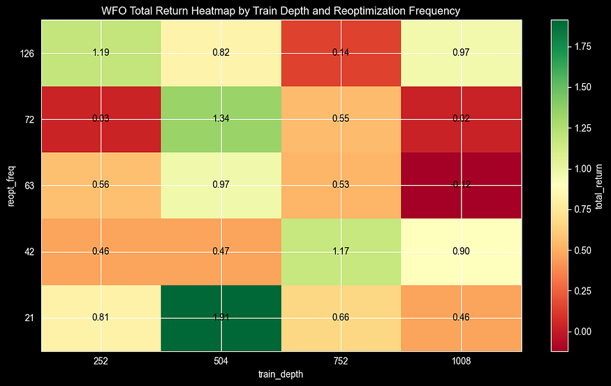
From this heatmap, we can understand various interesting facts:

• We have only one combination with a negative result, where we were optimising every 3 months using data from 4 years for training.
• Generally, it seems that four years of training are too much, capturing noise and producing the worst results.
• The best parameters are re-optimising every month, using data from the last 2 years. This resulted in a 190% return, which looks promising, especially considering that at the beginning of the article, we achieved 240% when testing our strategy with some basic short and long parameters (50 and 200) for the full period.

Final Thoughts

Walk-Forward Optimisation turns backtesting from a misleading guarantee into a practical assessment tool.

Key takeaways for your trading:

1. Never trust in-sample optimisation alone, as it’s almost always overfit.
2. WFO frequencies matter: Too frequent = noisy parameters; too infrequent = stale adaptation
3. Meta-optimisation reveals hidden truths (your “best” training window isn’t obvious)

Start with swapping random data for real FMP API calls, add transaction costs and slippage for institutional realism, then scale to multi-asset portfolios or even ML models. Deploy live by scheduling monthly reoptimisations with your optimal windows.

The code is production-ready. Copy it, adapt it, understand. Proper backtesting isn’t about finding the highest number. It’s about numbers that survive the future. You’ve got the toolkit. Now go build strategies that actually work.

What is Walk-Forward Backtesting? Implementation in Python was originally published in DataDrivenInvestor on Medium, where people are continuing the conversation by highlighting and responding to this story.