In the world of Machine Learning, there’s a common trap: believing that more data always equals a better model. We often dump every available column into our .fit() method, hoping the algorithm is "smart enough" to figure it out.

But here is the reality: Simple implementation is not enough for real-world scenarios. Irrelevant or redundant features introduce noise, lead to overfitting, and exponentially increase computational costs. This blog isn’t just about calling a library; it’s about understanding the “why” and “how” of Feature Selection (FS) from the ground up.
The Value Proposition: Why Feature Selection?
Before we dive into the math, let’s talk impact. Imagine training a model on 100 features versus 10 optimized ones.
- Accuracy: By removing noise, your model focuses on the true signal, often increasing precision.
- Interpretability: It’s easier to explain a model with 5 key drivers than 50 obscure variables.
- The “Curse of Dimensionality”: As the number of features increases, the data becomes sparse, making it harder for algorithms to find patterns.
Filter Methods: The Statistical Gatekeepers of Feature Selection
In machine learning, we often suffer from the “curse of dimensionality.” Adding every available feature to a model doesn’t just increase training time — it introduces noise that can degrade accuracy. Filter Methods act as the first line of defense, using statistical properties to score and rank features independently of any machine learning algorithm.
1. Variance Threshold: Eliminating the “Constants”
The simplest form of filtering is the Variance Threshold. The logic is straightforward: if a feature has zero or very low variance, it remains constant (or nearly constant) across all observations. Such a feature provides no predictive power because it doesn’t help the model distinguish between different classes or values.
The Code
# 1. Variance Threshold
print("--- Variance Threshold ---")
variances = X_df.var()
print("Variance of each feature:\n", variances)
selector_vt = VarianceThreshold(threshold=0.002)
selector_vt.fit(X_df)
selected_features_vt = X_df.columns[selector_vt.get_support()]
print(f"\nFeatures selected by Variance Threshold (threshold=0.002): {list(selected_features_vt)}")
- X_df.var(): We first calculate the variance of each column to understand the spread of the data.
- VarianceThreshold(threshold=0.002): We initialize the selector with a specific cutoff. Any feature with a variance below 0.002 will be flagged for removal.
- get_support(): This method returns a boolean mask indicating which features met the threshold. We use this to retrieve the final list of useful column names.
2. Correlation Coefficient: Tackling Redundancy
While Variance Threshold looks at features individually, the Correlation Coefficient looks at the relationship between a feature and the target variable. In a “Brute Force” approach, we also look for high correlation between two independent features (>0.95); if two features are nearly identical, one should be dropped to avoid redundancy.
The Code
# 2. Correlation Coefficient
print("\n--- Correlation Coefficient ---")
correlations = X_df.corrwith(pd.Series(y))
print("Correlation with target:\n", correlations)
- corrwith(): This Pandas function computes the pairwise correlation between the columns of the DataFrame and the target Series y.
- Significance: A high positive or negative correlation suggests a strong linear relationship. Features with correlations near zero are often candidates for removal as they lack a clear linear connection to the output.
3. Chi-Square Test: Association for Categorical Data
The Chi-Square (chi²) Test is specifically used to determine if there is a significant association between two categorical variables. It compares the “Observed” frequency in a contingency table to the “Expected” frequency if the variables were completely independent.
Mathematical Foundation
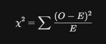
Where O is the observed frequency and E is the expected frequency.
The Code
# 3. Chi-Square Test
print("\n--- Chi-Square Test ---")
X_non_negative = X_df - X_df.min()
selector_chi2 = SelectKBest(score_func=chi2, k=5)
selector_chi2.fit(X_non_negative, y)
scores_chi2 = pd.Series(selector_chi2.scores_, index=feature_names)
p_values_chi2 = pd.Series(selector_chi2.pvalues_, index=feature_names)
print("Chi-Square scores:\n", scores_chi2)
print("\nChi-Square p-values:\n", p_values_chi2)
selected_features_chi2 = X_df.columns[selector_chi2.get_support()]
print(f"\nFeatures selected by Chi-Square (k=5): {list(selected_features_chi2)}")
- Preprocessing: X_df - X_df.min() ensures all data points are non-negative, a strict requirement for the Chi-Square calculation.
- SelectKBest: This is a wrapper that selects the top k features based on the chi2 score function.
- P-values: A low p-value (typically <0.05) indicates we can reject the null hypothesis of independence, meaning the feature is likely important for predicting the target.
4. Mutual Information: Capturing Complex Dependencies
Unlike correlation, which only detects linear relationships, Mutual Information (MI) measures the dependency between variables by capturing both linear and non-linear patterns. It quantifies how much information is shared between a feature and the target.
Mathematical Foundation
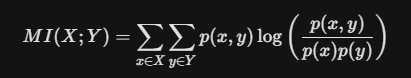
It calculates the difference between the joint distribution p(x, y) and the product of marginal distributions p(x)p(y).
The Code
# 4. Mutual Information
mi_scores = mutual_info_regression(X_df, y)
mi_scores_series = pd.Series(mi_scores, index=feature_names)
print("Mutual Information scores:\n", mi_scores_series.sort_values(ascending=False))
selector_mi = SelectKBest(score_func=mutual_info_regression, k=5)
selector_mi.fit(X_df, y)
selected_features_mi = X_df.columns[selector_mi.get_support()]
print(f"\nFeatures selected by Mutual Information (k=5): {list(selected_features_mi)}")
- mutual_info_regression: Specifically designed for continuous targets, it estimates MI using k-nearest neighbors methods.
- Interpreting Scores: A score of 0 means the variables are independent. Higher scores indicate stronger dependencies, whether they are linear, polynomial, or even more complex.
5. ANOVA F-test: Comparing Group Means
ANOVA (Analysis of Variance) is used to compare the means of samples to test the impact of factors on a continuous variable. It calculates the F-ratio to determine if the variation between group means is significantly larger than the variation within the groups.
Mathematical Foundation

The Code
# 5. ANOVA F-test
f_scores_anova, p_values_anova = f_regression(X_df, y)
f_scores_series = pd.Series(f_scores_anova, index=feature_names)
p_values_series = pd.Series(p_values_anova, index=feature_names)
print("ANOVA F-scores:\n", f_scores_series)
print("\nANOVA p-values:\n", p_values_series)
selector_anova = SelectKBest(score_func=f_regression, k=5)
selector_anova.fit(X_df, y)
selected_features_anova = X_df.columns[selector_anova.get_support()]
print(f"\nFeatures selected by ANOVA F-test (k=5): {list(selected_features_anova)}")
- f_regression: This function computes the F-score for each feature. It tests the individual effect of each feature on the target.
- Crucial Assumptions: For ANOVA results to be valid, the data should follow a normal distribution, have equal variance across groups, and remain independent of other observations.
Crucial Assumptions & Detection
Before relying on these filters, remember these statistical guardrails:
- Normality (ANOVA): Check using Q-Q plots or the Shapiro-Wilk test. If violated, consider transformations like Log or Box-Cox.
- Homogeneity of Variance: Use Levene’s test to ensure variance is consistent across groups.
- Independence: Ensure observations are not auto-correlated.
- Outliers: ANOVA and Correlation are highly sensitive to outliers. Use boxplots to detect and remedy them before filtering.
Wrapper Methods for Model-Optimal Feature Selection
In machine learning, we often mistake “more data” for “better performance.” However, irrelevant features act as noise, confusing our models and leading to overfitting. While statistical filters (like ANOVA) look at data in isolation, Wrapper Methods take a “model-aware” approach. They treat feature selection as a search problem, using a specific predictive model to evaluate and find the absolute best combination of columns.
The Core Framework: How Wrappers Work
Every wrapper method follows a recursive three-step cycle to arrive at the optimal feature subset:
- Subset Generation: The algorithm selects a specific combination of features to test.
- Subset Evaluation: A model is trained on this combination, and its performance is scored (e.g., R² or Accuracy).
- Stopping Criterion: The process repeats until a target number of features is reached or performance stops improving.
1. Exhaustive Feature Selection: The “Brute Force” King
Exhaustive selection is the most thorough method available. It evaluates every possible combination of features to identify the one that yields the highest score.
- The Logic: If you have features f_1, f_2, f_3, f_4, the algorithm will test subsets of size 1, 2, 3, and 4.
- Easy Example: Imagine you have 4 features. The algorithm tries all 2⁴ — 1 = 15 combinations.
- The Catch: The complexity is exponential (2^n), making it unsuitable for datasets with more than 15 columns.

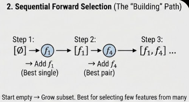
2. Sequential Forward Selection (SFS): The “Bottom-Up” Build
SFS is a greedy approach that starts with an empty set and adds one feature at a time.
- The Logic:
- Test every feature individually; pick the best (e.g., f_1).
- Pair f_1 with every remaining feature; pick the best pair (e.g., f_1, f_4).
- Continue until you reach the desired number of features.
- Easy Example: You have 100 features but only want the top 10. SFS is best here because it starts from zero and only needs 10 steps to reach its target.
3. Sequential Backward Elimination (SBE/SBS): The “Top-Down” Pruning
The inverse of SFS, this method starts with all features and removes the least useful one at each step.
- The Logic:
- Train a model on all features (f_1, f_2, f_3, f_4) and get a score (e.g., 0.89).
- Try removing one feature at a time. If removing f_3 increases the score to 0.91, drop f_3 permanently.
- Repeat until the score starts to drop or the target is met.
- Easy Example: If you have 100 features and want to keep 90, SBS is more efficient than SFS because it only needs to perform 10 “backwards” steps.

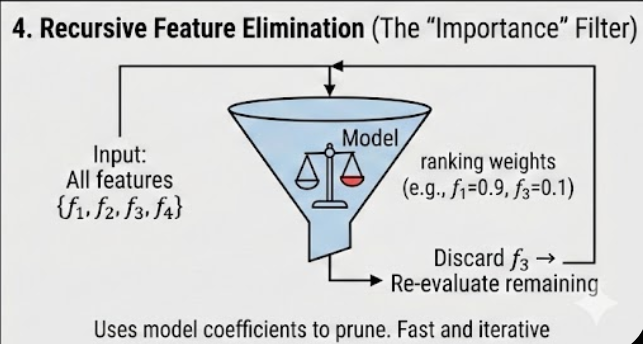
4. Recursive Feature Elimination (RFE): The Importance-Based Pruner
RFE is a sophisticated pruning method that uses a model’s internal feature importance (like coefficients) to rank and remove features.
- The Logic:
- Train the model on all features.
- Calculate feature importance rankings (e.g., coefficients for Linear Regression).
- Remove the feature with the lowest ranking (least importance).
- Re-train the model on the remaining features and repeat.
- Easy Example: Imagine a model assigns weights: f_1=0.8, f_2=0.5, f_3=0.1. RFE instantly flags f_3 for removal, then re-evaluates f_1 and f_2 to see how their weights change.
Python Implementation: Bringing it to Life
Using Scikit-Learn, we can implement both RFE and SFS efficiently using any standard estimator like LinearRegression.
Python
from sklearn.feature_selection import RFE, SequentialFeatureSelector
from sklearn.linear_model import LinearRegression
# Initialize the base model (The "Wrapper")
estimator = LinearRegression()
# 1. Implement Recursive Feature Elimination (RFE)
rfe = RFE(estimator, n_features_to_select=5)
rfe.fit(X_df, y)
selected_features_rfe = X_df.columns[rfe.get_support()]
print("Features selected by RFE:", list(selected_features_rfe))
# 2. Implement Sequential Feature Selector (SFS)
# By default, this uses Forward selection to reach 5 features
sfs = SequentialFeatureSelector(estimator, n_features_to_select=5)
sfs.fit(X_df, y)
selected_features_sfs = X_df.columns[sfs.get_support()]
print("Features selected by SFS:", list(selected_features_sfs))
The “Crucial Assumptions” & Risks
While Wrapper methods are highly accurate, they come with a high Overfitting Risk. Because the feature subset is “tuned” specifically for one model, the selection might not generalize well to other models or unseen data.
- The Remedy: Always use Cross-Validation (like RFECV) to ensure the feature importance is stable across different subsets of your training data.
- The Stopping Rule: In libraries like mlxtend, the process stops if the score doesn't improve, whereas sklearn typically requires a fixed number of features.
The Efficiency of Embedded Methods
In machine learning, the goal is often simplicity and precision. While Filter methods use statistics and Wrapper methods use brute-force searching, Embedded methods integrate feature selection directly into the model construction process. By doing so, they solve the limitations of both previous approaches — capturing feature interactions while remaining computationally efficient.
In this blog, we’ll dive deep into the math and implementation of embedded methods, from linear regularization to tree-based importance.
1. Mathematical Foundation: The Penalty Terms
Embedded methods primarily rely on Regularization, which adds a penalty term to the loss function (typically Mean Squared Error) to discourage complex models with large or irrelevant coefficients.
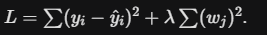
A. Lasso Regression (L1 Regularization)
Lasso (Least Absolute Shrinkage and Selection Operator) is the definitive embedded selection tool because it encourages sparsity — driving the coefficients of unimportant features exactly to zero.
- Formula:

- Mechanism: The L1 penalty creates a “diamond-shaped” constraint in feature space, making it highly likely for the optimal weights to land on an axis, thus zeroing them out.
B. Ridge Regression (L2 Regularization)
Ridge shrinks coefficients toward zero but, unlike Lasso, it rarely sets them to exactly zero. It helps reduce model complexity and handles multicollinearity but does not perform feature selection in the strictest sense.
- Formula:
3. Library Comparison: Using Scikit-Learn
In production, we use the SelectFromModel meta-transformer to automate the selection based on these internal model weights.
from sklearn.linear_model import Lasso, Ridge, ElasticNet
from sklearn.feature_selection import SelectFromModel
from sklearn.ensemble import RandomForestRegressor
# Initialize the embedded models
lasso = Lasso(alpha=0.1, random_state=42)
ridge = Ridge(alpha=0.1, random_state=42)
elastic_net = ElasticNet(alpha=0.1, l1_ratio=0.5, random_state=42)
rf_regressor = RandomForestRegressor(n_estimators=100, random_state=42)
# 1. Selection with Lasso (Coefficient-based)
selector_lasso = SelectFromModel(lasso)
selector_lasso.fit(X_df, y)
selected_lasso = X_df.columns[selector_lasso.get_support()]
print("Features selected by Lasso:", list(selected_lasso))
# 2. Selection with Random Forest (Impurity-based)
# Trees inherently rank features based on their ability to split data
selector_rf = SelectFromModel(rf_regressor)
selector_rf.fit(X_df, y)
selected_rf = X_df.columns[selector_rf.get_support()]
print("Features selected by Random Forest Importance:", list(selected_rf))
4. The “Crucial Assumptions” Section
Before deploying embedded methods, ensure these criteria are met to avoid misleading results:
- Scaling is Mandatory: For Lasso and Ridge, you must standardize your features (mean=0, variance=1). Because the penalty is applied to the magnitude of the coefficients, features with larger raw scales will be unfairly penalized.
- Linearity (for Regularized Models): Lasso and Ridge assume a linear relationship between features and the target.
- No Strong Multicollinearity for Lasso: If two features are highly correlated, Lasso might randomly pick one and discard the other. Use Elastic Net if your features are highly interdependent.
5. Visual Interpretation Guide
- The Lasso Path: Plotting your coefficients against the value of lambda (alpha) is the best way to visualize selection. You will see lines representing different features “hit” the zero axis as lambda increases.
- Feature Importance Bars: For tree-based methods, use a bar chart to show Impurity Decrease. Features with scores below the average importance (threshold=’mean’) are typically the ones pruned.
Let’s Connect!
- LinkedIn: pruthil-prajapati
- Email: Gmail
- GitHub: Pruthil-2910
Keep exploring the math behind the models!
#BuildInPublic #ArtificialIntelligence #DataEngineering #SoftwareEngineering #Mathematics #ProgrammingTips #100DaysOfCode #UnderTheHood #MathForML #FromScratch #CodeNewbie #Vectorization #Optimization #AlgorithmDesign #NumPy #Python
The Secret Sauce of Model Performance: A Deep Dive into Feature Selection was originally published in Level Up Coding on Medium, where people are continuing the conversation by highlighting and responding to this story.