Finding the UX ceiling of local analytics on low-end hardware with a 50M row benchmark.
DuckDB shouldn’t work this well. It’s a single embedded library that needs no server, config, or cloud bill — yet it handles warehouse-scale columnar analytics with surprising ease.
Plenty of benchmarks already show that DuckDB can process large datasets. The more useful question, to me, is narrower: how far does it scale on low-end hardware before interactivity breaks down? I do data forensics for a living, and the last thing I want is infrastructure getting in the way.
To answer that, I ran a 50-million-row benchmark on a ~$500 Acer Aspire 5 (Raptor Lake i5, 16GB RAM, 1 TB SSD). Starting with 50,000 real-world search results, I generated a large synthetic dataset and executed increasingly complex analytical queries to identify where performance crossed practical thresholds.
I’ll present my findings here. The result wasn’t a catastrophic failure point, but a series of predictable transitions (from instant, to tolerable, to better-scheduled-than-waited-on) depending on query shape.
Table of Contents
- The Four Performance Zones
- The Goldilocks Zone for Local Analytics
- Memory is Not the Bottleneck
- Window Functions Affect Scaling the Most
- …But Make Sure You Checkpoint Enough
- Methodology — How the Benchmark Was Built
- Limitations of this Study
- Conclusion — Scaling Is a UX Ceiling
1. The Four Performance Zones
Before I dive into specific query types, understand that not all scales perform the same way. The same query that feels instant at 1 million rows might cross into “go grab a coffee” territory at 30 million — and different query types degrade at different rates.
So there isn’t one big scale — but three. One for each type of analytical query:
- Percentile queries (likeGROUP BY + PERCENTILE_CONT) — when you’re trying to answer questions like “For each domain, what’s its median, 25th, 75th, and 95th percentile search ranking?” Or: “For each customer tier, what is the session duration distribution?” This is the kind of query you run when averages aren’t enough. You want to understand spread, skew, and outliers. It’s common in finance, product analytics, marketplace reporting — anywhere distributions matter more than single numbers.
- Window functions (likeLAG with PARTITION BY) — e.g. “For each user, how did their activity change vs. previous session?” Or: “For each account, how did monthly revenue change vs. last month?” This is bread-and-butter analytics — a simple time-series comparison. It’s what powers growth dashboards, churn analysis. Amazon, for example, uses this extensively for anomaly detection. These are more expensive because they require partitioning and sorting — especially on large datasets like ours.
- Aggregations (likeCOUNT, AVG, MIN, MAX with DISTINCT) — e.g. “For each region, how many total orders did we ship, how many unique customers/products, what were the min/max purchase values?” This is the classic summary view, the kind of query behind almost every dashboard card. Deceptively simple because DISTINCT at scale forces the engine to work harder than you might expect.
Together, these three queries make up a massive chunk of all real-world analytics.
Here’s how they perform going from 1,000 to 50,000,000 rows:
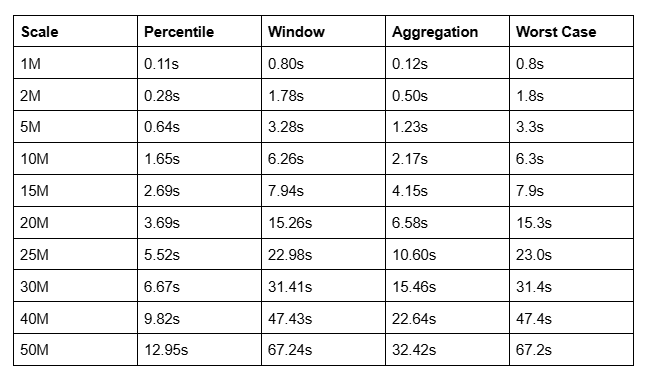
| Scale | Percentile | Window | Aggregation | Worst Case |
| :---- | :---- | :---- | :---- | :---- |
| 1M | 0.11s | 0.80s | 0.12s | 0.8s |
| 2M | 0.28s | 1.78s | 0.50s | 1.8s |
| 5M | 0.64s | 3.28s | 1.23s | 3.3s |
| 10M | 1.65s | 6.26s | 2.17s | 6.3s |
| 15M | 2.69s | 7.94s | 4.15s | 7.9s |
| 20M | 3.69s | 15.26s | 6.58s | 15.3s |
| 25M | 5.52s | 22.98s | 10.60s | 23.0s |
| 30M | 6.67s | 31.41s | 15.46s | 31.4s |
| 40M | 9.82s | 47.43s | 22.64s | 47.4s |
| 50M | 12.95s | 67.24s | 32.42s | 67.2s |
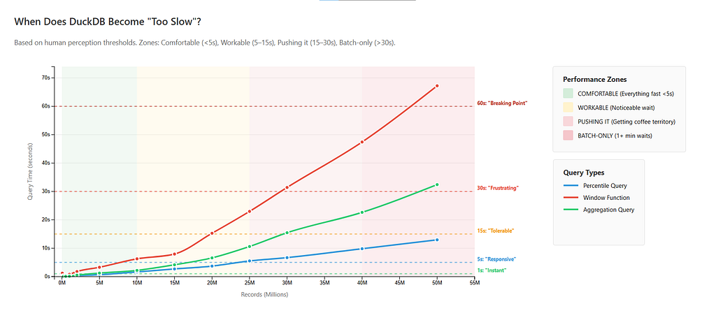
Having plotted query times against human perception thresholds (I made some assumptions for those, since this is subjective), we have four distinct performance zones — with boundaries shifting depending on which query type you care about.
“Comfort Zone”: Up to 5M Records
Query times: Near instantaneous, < 3 seconds for everything.
This is why DuckDB feels magical. For everything up to 5 million rows (and let’s be honest — more data than most organizations are querying interactively anyway) — all queries are fast. Window functions complete in under a second at 1M. Even at 5M rows, the slowest query (you guessed it; a window function) takes just 3.3 seconds. Percentiles and aggregations are sub-second through 2M and barely crack 1 second at 5M.
At this scale, DuckDB keeps everything comfortably in memory. Hash tables fit in RAM, partitioning operations don’t require temp files, and there’s zero disk spilling. This is the sweet spot for team analytics, dashboards, and interactive data exploration.
“Workable”: 5–20M Records
Query times:
- Window functions: 3–15 seconds. Noticeable latency. At 10M they take 6 seconds, and at 15M, about 8 seconds. They hit 15 seconds right at 20M — the upper edge of this zone.
- Percentiles and aggregations: still under 4 and 7 seconds respectively.
This is where window queries will make people Alt-Tab out to do something else — doomscroll, check their email, watch videos of cats — instead of waiting. Percentiles and aggregations are still firmly comfortable, though.
This zone is still good for Data science work and one-off analyses where a 10–15 second wait is acceptable. Still no disk spilling. Memory usage stays under ~650 MB.
“Now You’re Pushing It”: 20–30M Records
Query times:
- Window functions: 15–31 seconds, always crossing the 15s “frustration threshold”.
- Aggregations: 7–15 seconds (10.6s at 25M, 15.5s at 30M), near-annoying latency now.
- Percentiles: 4–7 seconds (5.5s at 25M, 6.7s at 30M.)
This is the point where query types diverge dramatically. Percentiles are still firmly in the “interactive” category, but aggregations require patience. Window functions however, are firmly in the “go do something else” territory — at 30M records, they can reach a whopping 31 seconds — clearly the point where you should batch these, instead of waiting live.
In general, this zone is best for automated/scheduled work where humans aren’t waiting on complex queries. Simple aggregations and percentiles are still interactive enough.
“Batch-Only”: 30M+ Records
Query times:
- Window functions: 31–67 seconds. Always past one minute at 50M.
- Aggregations: 15–32 seconds. Always past 30 seconds at 50M.
- Percentiles: 7–13 seconds.
In a testament to how performant DuckDB can be — if you’re only running percentiles, even 50M rows is still marginally interactive (tops out at 13 seconds.)
Everything else at this scale, though, should be scheduled.
If you need window functions, this (30M and above) is clearly the point where you should consider a cloud data warehouse — they cross a minute at 50M (~67 seconds). Aggregations taking 20–30 seconds on average is also beyond generous definitions of “interactive”.
So this is where we’ve found our limit — albeit not a hard one. Performance degrades predictably, not catastrophically. Critically, there’s still zero disk spilling. DuckDB never writes temp files to disk, even at 50M records. Memory usage peaked at ~1.2 GB.
Here’s a practical cheatsheet, sorted by use case:
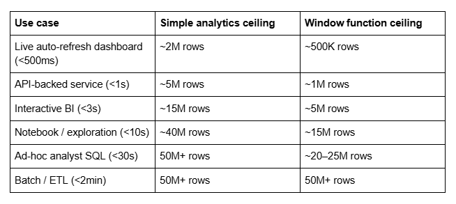
| Use case | Simple analytics ceiling | Window function ceiling |
| :---- | :---- | :---- |
| Live auto-refresh dashboard (<500ms) | ~2M rows | ~500K rows |
| API-backed service (<1s) | ~5M rows | ~1M rows |
| Interactive BI (<3s) | ~15M rows | ~5M rows |
| Notebook / exploration (<10s) | ~40M rows | ~15M rows |
| Ad-hoc analyst SQL (<30s) | 50M+ rows | ~20–25M rows |
| Batch / ETL (<2min) | 50M+ rows | 50M+ rows |
2. The Goldilocks Zone for Local Analytics
If I had to draw a circle around the scale where DuckDB on a cheap laptop is just right — fast enough to feel interactive, complex enough to handle real analytical work, without needing to think about infrastructure — it’s 1M to 10M rows.
Here’s why that range is special.
At 1M rows, every query type is effectively instant. Aggregations finish in 0.06 seconds. Even the most expensive query in the test — the LAG window function — takes 0.47 seconds. The database is not part of your cognitive load at all at this scale.
At 5M rows, that’s still largely true. Aggregations take half a second. Percentiles take 1.3 seconds. Window functions take 1.7 seconds. 5M rows of real data is a meaningful dataset — a year of event logs for a mid-sized SaaS product, a full crawl of a large website, several years of transaction history for a small business. And DuckDB chews through it without complaint.
At 10M rows, you start paying a tax specifically on window functions — they cross 6 seconds here. But aggregations (0.79s) and percentiles (1.99s) are still fast enough that interactive use feels natural. If your workload skews toward GROUP BY analytics and distribution queries rather than time-series comparisons, 10M rows is still firmly comfortable.
So our “Goldilocks” Zone — so named after the fairytale of Goldilocks and the Three Bears; Goldilocks rejects porridges that are too hot and too cold, until finding one that’s “just right” — is up to ~10M rows for any query type, and up to ~20M rows if you’re willing to accept that window functions will make you wait.
Below that ceiling, DuckDB on cheap/commodity hardware is no compromise at all.
3. Memory is Not the Bottleneck
Across all scales tested (1K → 50M rows, averaged over 5 runs) DuckDB never exceeded ~1.2 GB of memory — even at 50 million rows.

At the upper bound (50 million rows), peak observed memory usage was ~1,212 MB. On my 16GB laptop that’s ~7.5%. And that’s the worst case in this benchmark — with 50M rows and window-heavy queries in play.
Memory growth is real — especially with window function (delta) queries — but it’s still fairly controlled, I’d say:
- 10M rows → ~600 MB range
- 20M rows → ~650 MB range
- 30–50M rows → ~900 MB–1.2 GB range
Time, on the other hand, accelerates sharply:
- Window query: ~6.4s at 10M
- ~15.8s at 20M
- ~70s at 50M
So the practical ceiling on a cheap laptop isn’t RAM. You’ll run out of patience before you run out of memory. It means for many local analytics use cases the scaling limit is UX, not hardware — that’s a very different kind of bottleneck, though.
Before we move on, an interesting thing to note is that the aggregation query degrades faster than percentiles at scale. At 5M they’re similar (~0.6s vs ~1.2s), but by 50M the aggregation (33.7s) is nearly 3x the percentile (12.5s). Multi-metric GROUP BY with HAVING and DISTINCT counts WILL get expensive. If your dashboard runs heavy aggregations specifically, you should probably discount the “simple” ceiling by ~30–40%.
4. Window Functions Affect Scaling The Most
If you’re embedding DuckDB in:
- A local analytics tool
- A CLI data processor
- A desktop SaaS product
- A developer-facing data tool
Row count alone is not your sizing variable. Query shape is.
Across 18 dataset scales (1k → 50M rows, averaged over 5 runs, the single biggest performance divider wasn’t how much data existed — it was whether the workload used window functions, at all.
Window functions power extremely common patterns:
- Ranking results per group (RANK(), ROW_NUMBER())
- Comparing rows over time (LAG(), LEAD())
- Running totals
- Sessionization
- Deduplication
These are all operations you’ll run many, many times for a real project.
I found that on identical hardware, aggregation-heavy workloads comfortably scale to tens of millions of rows while staying interactive. These Window-heavy workloads, though, hit “coffee break” territory much earlier.
At 10M rows
- Percentile query (aggregation-heavy): ~1.7s, ~217 MB memory delta
- Window “delta” query (LAG-style): ~6.4s, ~46 MB memory delta
- Group aggregation: ~2.5s, ~200 MB memory delta
Already, the window query is ~3–4x slower than pure aggregation.
At 20M rows
- Percentile: ~4.1s
- Window (delta): ~15.8s
- Aggregation: ~7.3s
The gap widens. The window query is now roughly 2–4x slower than aggregation-style queries.
At 50M rows
- Percentile: ~16.5s, ~330 MB delta
- Window (delta): ~70.3s, ~588 MB delta
- Aggregation: ~33.3s, ~113 MB delta
This is where the separation becomes untenable:
- The window query takes 70 seconds.
- Aggregation-heavy queries remain roughly half that.
- Memory growth for window logic accelerates much more aggressively at scale.
If your workload is mostly GROUP BY, percentiles, and simple scans, then you have substantial headroom. If your workload relies heavily on LAG(), LEAD(), RANK() OVER (PARTITION BY …) then your practical ceiling with DuckDB (running on such consumer grade local hardware, at least) arrives much sooner.
5. …But Make Sure you Checkpoint Enough
Speaking of window functions, avery interesting recurring pattern I found was that at exactly 50,000 records, these hit a wall.

This pattern is consistent across all 5 runs:
- 20K records: 0.24 seconds (fast)
- 50K records: 1.21 seconds (5x slower than expected)
- 100K records: 0.20 seconds (fast again)
This specific spike appears in every single run with CV (coefficient of variation) of only 10.3%. Expected time based on linear scaling was 0.23 seconds. Actual time? 1.21 seconds. That’s 430% slower than it should be!
It’s the only non-monotonic performance pattern in the entire dataset. Every other scale shows smooth, predictable scaling. The 50K spike for window/delta functions is the exception.
Why it happens: Checkpoint more frequently. DuckDB has automatic checkpointing (wal_autocheckpoint), but it doesn’t work reliably during bulk inserts from Python. (Check this GitHub issue). Knowing this, I set checkpointing manually, but as it turned out I wasn’t checkpointing enough.
Data was inserted in 1,000-row batches across multiple database connections, but I had a LOT of records (50 million) so I thought I’d manually trigger CHECKPOINT only every 100K rows.
💡 CHECKPOINT is a database operation that flushes pending writes to disk and optimizes storage layout. In DuckDB specifically:
- Consolidates fragmented columnar segments created by many small inserts
- Reorganizes data into optimized columnar format for faster reads
- Flushes the write-ahead log (WAL) to the main database file
Like defragmenting a hard drive, CHECKPOINT reorganizes scattered data into contiguous, optimized blocks.
Because the scales were run sequentially (1K → 5K → 10K → 20K → 50K → 100K and so on), by the time the 50K test executed, dozens of small batch inserts had accumulated without a CHECKPOINT, leaving the write-ahead log fragmented across many small column segments.
Now consider the query that spikes:
LAG(rank) OVER (PARTITION BY url, query ORDER BY timestamp)
This requires a full sort of the relevant partitions. Sorting is exactly the kind of operation that is most sensitive to storage layout, and fragmented column segments mean less efficient scanning and sorting. So at 50K, the query pays the fragmentation penalty.
By 50K I had 50 fragmented segments. The window function’s sort pays the cost of reading across all those fragments. At 100K, CHECKPOINT compacted everything, so queries got faster despite more data.
That’s all the data I found. If you want to know about my methodology for this (admittedly) very niche benchmark, read on.
Methodology — How this Low-End Benchmark Was Built
What I wanted to do was stress-test DuckDB with realistic analytical queries at scales most teams would consider “cloud warehouse only.” So if I wanted to benchmark how it performed on low-end hardware, I had to flip the entire approach on its head.
Step 1 — Getting Search Data
I started by fetching 50,000 actual Google SERP results using Bright Data’s SERP API. Why SERP data? Because search results have realistic cardinality — lots of unique URLs, domains, queries, timestamps — exactly the kind of data that stresses analytical databases.
I built ~2,550 unique queries by combining 50 base topics with 51 suffix variations:
_BASE_TOPICS = [
    "python programming",
    "machine learning",
    "web development",
    # ... 47 more
]

_QUERY_SUFFIXES = [
    "",
    " tutorial",
    " 2024",
    " best practices",
    # ... 47 more
]

SERP_QUERIES = [
    f"{base}{suffix}".strip()
    for base in _BASE_TOPICS
    for suffix in _QUERY_SUFFIXES
]
SERP_QUERIES = list(dict.fromkeys(SERP_QUERIES))
Full code here: serp_queries.py
Each query fetched up to 20 organic results via the API, streamed directly into DuckDB as results came in:
client = BrightDataClient()

with DuckDBManager() as db:
    while results_obtained < total_results:
        query = queries[query_idx % len(queries)]
        serp_data = client.search(query, num_results=batch_size)

        organic_results = []
        if isinstance(serp_data, dict):
            if 'organic' in serp_data:
                organic_results = serp_data['organic']
            elif 'body' in serp_data and isinstance(serp_data['body'], dict):
                if 'organic' in serp_data['body']:
                    organic_results = serp_data['body']['organic']

        if organic_results:
            db.insert_batch(organic_results, query)
            results_obtained += len(organic_results)

        query_idx += 1
        time.sleep(delay_seconds)
Full code here: bright_data.py
My DuckDB schema mirrors the SERP data structure the API returns. (Check their docs here for more info):
self.conn.execute("""
    CREATE TABLE IF NOT EXISTS serp_results (
        id BIGINT PRIMARY KEY,
        query TEXT NOT NULL,
        timestamp TIMESTAMP NOT NULL,
        result_position INTEGER NOT NULL,
        title TEXT,
        url TEXT,
        snippet TEXT,
        domain TEXT,
        rank INTEGER,
        previous_rank INTEGER,
        rank_delta INTEGER
    )
""")
Full code here: duckdb_manager.py
This adds up to 50K rows of real, varied data with natural patterns — not artificial test data…but that still wasn’t enough.
Step 2 — Synthesize 50M Records from Real Patterns
50K rows isn’t enough to stress-test at scale. But completely random synthetic data loses the realistic patterns that make queries slow. So I extracted actual domains, queries, title structures, and snippets from the real data and used those to generate variations:
def extract_serp_patterns(db_path):
    with DuckDBManager(db_path) as db:
        queries = db.conn.execute(
            "SELECT DISTINCT query FROM serp_results ORDER BY RANDOM() LIMIT 100"
        ).fetchall()
        domains = db.conn.execute(
            "SELECT DISTINCT domain FROM serp_results WHERE domain IS NOT NULL LIMIT 200"
        ).fetchall()
        title_samples = db.conn.execute(
            "SELECT title FROM serp_results WHERE title IS NOT NULL LIMIT 50"
        ).fetchall()
        snippet_samples = db.conn.execute(
            "SELECT snippet FROM serp_results WHERE snippet IS NOT NULL LIMIT 50"
        ).fetchall()
        return {
            'queries': [r[0] for r in queries],
            'domains': [r[0] for r in domains],
            ...
        }
Synthetic rows were generated in batches of 10,000 and inserted directly, mixed in with the 50k real records, until we had 50M total:
for i in range(0, needed, batch_size):
    batch = [{
        'id': current_id,
        'query': random.choice(queries),
        'domain': random.choice(domains),
        ...
    } for j in range(batch_size)]
    df = pd.DataFrame(batch)
    db.conn.execute("INSERT INTO serp_results SELECT * FROM df")
Full code here: benchmark.py
Step 3 — Design the Query Suite
I chose three query types that represent common analytical workloads:
Percentile Queries:
query = f"""
    SELECT
        domain,
        COUNT(*) as result_count,
        AVG(rank) as avg_rank,
        PERCENTILE_CONT(0.5) WITHIN GROUP (ORDER BY rank) as median_rank,
        PERCENTILE_CONT(0.25) WITHIN GROUP (ORDER BY rank) as p25_rank,
        PERCENTILE_CONT(0.75) WITHIN GROUP (ORDER BY rank) as p75_rank,
        PERCENTILE_CONT(0.95) WITHIN GROUP (ORDER BY rank) as p95_rank
    FROM serp_results
    {where_clause}
    GROUP BY domain
    ORDER BY avg_rank
    LIMIT 100
"""
Window Functions:
query = f"""
    WITH ranked AS (
        SELECT
            url,
            query,
            rank,
            timestamp,
            LAG(rank) OVER (PARTITION BY url, query ORDER BY timestamp) as previous_rank
        FROM serp_results
        {id_filter}
    )
    SELECT
        url,
        query,
        rank,
        previous_rank,
        rank - previous_rank as rank_delta,
        timestamp
    FROM ranked
    WHERE previous_rank IS NOT NULL
    ORDER BY ABS(rank_delta) DESC
    LIMIT 100
"""
Aggregation Queries:
query = f"""
    SELECT
        domain,
        COUNT(*) as total_results,
        COUNT(DISTINCT query) as unique_queries,
        AVG(rank) as avg_rank,
        MIN(rank) as best_rank,
        MAX(rank) as worst_rank,
        COUNT(DISTINCT url) as unique_urls
    FROM serp_results
    {where_clause}
    GROUP BY domain
    HAVING COUNT(*) > 10
    ORDER BY total_results DESC
    LIMIT 50
"""
Full code (all queries) here: queries.py
These test different bottlenecks: percentiles stress sorting and statistical aggregation; window functions stress partitioning and stateful operations; aggregations stress hash tables and DISTINCT operations.
Step 4 — Run at 18 Different Scales
Instead of regenerating data for each scale, I used a single optimization: filter by ID. One dataset, 18 different windows into it:
max_id_result = db.conn.execute(f"""
    SELECT id FROM (
        SELECT id FROM serp_results ORDER BY id LIMIT {target_count}
    ) ORDER BY id DESC LIMIT 1
""").fetchone()

max_id = max_id_result[0]
Every query then receives this max_id as a filter:
where_clause = f"WHERE id <= {max_id} AND domain IS NOT NULL AND domain != ''"Full code here: benchmark.py
This tested 1K, 5K, 10K, 20K, 50K, 100K, 200K, 500K, 1M, 2M, 5M, 10M, 15M, 20M, 25M, 30M, 40M, and 50M records against identical data — isolating row count as the only variable. Each scale measured query execution time and peak memory usage via psutil.
Step 5 — Run Five Complete Iterations
To ensure patterns weren’t random variance, I ran the entire benchmark suite five times. This produced 90 data points per query type (5 runs × 18 scales).
The result: performance was shockingly consistent. Most metrics had <10% coefficient of variation across runs — the 50M window function result, for instance, varied by less than 1 second across all five runs.
Limitations
- Uniform synthetic distribution: The 50M records were generated by sampling uniformly from ~200 real domains and ~100 real queries. Real-world data follows a power-law distribution — a small number of domains dominate traffic heavily. This means the PARTITION BY url, query window function hits roughly equal-sized partitions in this benchmark, which is best-case behavior. In production data with skewed distributions, window function performance at scale could be meaningfully worse than the numbers here suggest.
- Single-table queries only: Didn’t test multi-table joins or recursive CTEs.
- Hardware-specific: Tested on one machine (16GB RAM). Results may vary on different hardware.
- Query-specific: These three query types don’t represent all analytical workloads.
- DuckDB version: Tested on DuckDB >=1.0.0. Newer versions may perform differently.
- No concurrent queries: Single-threaded only, no concurrent workload tested.
Conclusion — Scaling Is a UX Ceiling.
This experiment was more about finding out where local analytics on consumer grade hardware stops feeling interactive, rather than stress-testing DuckDB.
Across all runs, DuckDB remained stable and memory usage stayed modest. There was no hard failure point, no dramatic collapse in performance. Instead, execution times increased predictably as data grew — and different query shapes crossed the interactivity threshold at different scales. Aggregation-heavy workloads retained responsiveness far longer, while window-heavy queries reached the UX ceiling much sooner.
This, then, is our practical takeaway: the limiting factor on local analytics isn’t usually RAM or disk; it’s the point at which queries stop feeling fluid. At that boundary, the decision you have to make is entirely about whether (for your use case) the user experience is still good enough to keep things local.
Some links in this article are tracking links used for analytics purposes only. I do not receive any commission or compensation from them.
The Practical Limits of DuckDB on Commodity Hardware was originally published in Level Up Coding on Medium, where people are continuing the conversation by highlighting and responding to this story.

