
Attention gets the headlines. But between every attention block, two quieter operations do the real work of keeping Transformers stable and expressive: Layer Normalization and the Feed-Forward Network.
My previous articles covered how embeddings convert words into vectors, how positional encoding adds word order, and how attention lets every word gather context from every other word. But attention alone is not enough to build a working Transformer.
Between every attention block, two operations happen that rarely get discussed but are essential: Layer Normalization stabilizes the numbers flowing through the model, and the Feed-Forward Network gives each word its own independent transformation. Without these two components, Transformers would either collapse during training or lack the expressive power to model complex language.
This article breaks down both, what they do, why they exist, and how they work in code.
Part 1: Layer Normalization: Keeping the Numbers Under Control
The Problem: Numbers That Grow Too Big or Shrink Too Small
A Transformer is deep, meaning it has many layers stacked on top of each other. BERT has 12. GPT-3 has 96. At each layer, the numbers inside every word’s embedding get multiplied, added, and transformed. This happens again and again, layer after layer.
Here is the issue: when you keep multiplying numbers together many times, one of two things tends to happen.
The numbers explode. Imagine multiplying 1.1 × 1.1 × 1.1… a hundred times. You get a huge number. The same thing happens inside the model , values that started small can balloon into thousands or millions after dozens of layers. When numbers get that large, the math breaks down and the model stops learning.
The numbers vanish. Now imagine multiplying 0.9 × 0.9 × 0.9… a hundred times. You get something extremely close to zero. When all the values shrink toward zero, every word looks the same to the model, and it can no longer tell “cat” from “democracy.”
This is not a hypothetical worry. It is the core reason why deep networks were historically so difficult to train, and it is exactly the problem Layer Normalization was designed to solve.
The Solution: Layer Normalization
What Layer Normalization Does
Think of it like adjusting the brightness and contrast on a photo. The photo (the embedding) has all its important information, it might just be too bright or too dark to see clearly. Normalization adjusts the scale so everything is in a readable range, without changing what the photo actually shows. Specifically, Layer Normalization takes a word’s embedding vector and rescales it so that the values have a mean (average) of 0 and a standard deviation of 1. In other words, Layer normalization normalizes across the embedding dimensions of a single token, not across tokens in a batch. Then it applies two small learned adjustments, gamma (scale) and beta (shift), that let the model fine-tune the result to whatever works best.

Don’t worry about memorizing the formula. Here is what matters:
- x is the input: one word’s embedding vector
- mean and variance are calculated from the values in that vector
- gamma and beta are parameters the model learns during training
- epsilon is a tiny number (like 0.00001) just to avoid dividing by zero
import numpy as np

def layer_norm(x, gamma, beta, epsilon=1e-5):
    """
    x: input vector (d_model,)
    gamma: learned scale parameter (d_model,)
    beta: learned shift parameter (d_model,)
    """
    mean = np.mean(x)
    variance = np.var(x)

    # Normalize to mean=0, std=1
    x_normalized = (x - mean) / np.sqrt(variance + epsilon)

    # Scale and shift with learned parameters
    output = gamma * x_normalized + beta

    return output, mean, variance

# Simulate an embedding vector that has drifted to large values
np.random.seed(42)
d_model = 8  # small for demonstration

# An embedding vector with problematic scale
x = np.array([150.2, -89.5, 230.1, -45.3, 178.9, -120.4, 95.7, -200.1])

# Learned parameters (initialized to gamma=1, beta=0 in practice)
gamma = np.ones(d_model)
beta = np.zeros(d_model)

output, mean, var = layer_norm(x, gamma, beta)

print("Before Layer Normalization:")
print(f"  Values: {x}")
print(f"  Mean: {mean:.2f}")
print(f"  Std: {np.std(x):.2f}")
print(f"  Range: [{x.min():.1f}, {x.max():.1f}]")

print("\nAfter Layer Normalization:")
print(f"  Values: {output.round(3)}")
print(f"  Mean: {output.mean():.6f}")
print(f"  Std: {output.std():.4f}")
print(f"  Range: [{output.min():.3f}, {output.max():.3f}]")
Before Layer Normalization:
  Values: [ 150.2  -89.5  230.1  -45.3  178.9 -120.4   95.7 -200.1]
  Mean: 24.95
  Std: 148.45
  Range: [-200.1, 230.1]

After Layer Normalization:
  Values: [ 0.844 -0.771  1.382 -0.473  1.037 -0.979  0.477 -1.516]
  Mean: -0.000000
  Std: 1.0000
  Range: [-1.516, 1.382]
Before normalization, values range from -200 to 230, way too spread out. After normalization, they are neatly centered around 0 with a standard deviation of 1. The important part: the relative relationships are preserved. The largest value is still the largest, the smallest is still the smallest. The information is intact, it’s just at a manageable scale now.
Why Not Batch Normalization?
If normalization sounds familiar, it might be because of Batch Normalization, a technique widely used in image models. They sound similar but work differently.
The easiest way to understand the difference:
Batch Normalization looks at the same dimension across many different examples. It asks: “Across all 64 sentences in this batch, what is the average value of dimension 47?”
Layer Normalization looks at all dimensions within a single example. It asks: “For this one word’s embedding, what is the average value across all 768 dimensions?”
Why does this matter for Transformers? Sentences come in different lengths. A batch might have a 5-word sentence next to a 50-word sentence. Comparing the same position across such different sentences does not make much sense. Layer Normalization avoids this problem entirely, it normalizes each word on its own, regardless of what other sentences are in the batch.
import matplotlib.pyplot as plt

fig, axes = plt.subplots(1, 2, figsize=(14, 5))

# Create sample data: batch of 4 sentences, each with 6-dimensional embeddings
batch = np.random.randn(4, 6) * 10 + 5

# Batch Normalization: normalize down columns
ax1 = axes[0]
ax1.imshow(batch, cmap="RdBu", aspect="auto")
ax1.set_xlabel("Embedding Dimension", fontsize=11)
ax1.set_ylabel("Example in Batch", fontsize=11)
ax1.set_title("Batch Normalization\nNormalizes down each column (across examples)", fontsize=12)
ax1.set_xticks(range(6))
ax1.set_yticks(range(4))
ax1.set_yticklabels(["Sentence 1", "Sentence 2", "Sentence 3", "Sentence 4"], fontsize=9)

for j in range(6):
    ax1.annotate('', xy=(j, 3.4), xytext=(j, -0.4),
                arrowprops=dict(arrowstyle='->', color='black', lw=1.5))

# Layer Normalization: normalize across rows
ax2 = axes[1]
ax2.imshow(batch, cmap="RdBu", aspect="auto")
ax2.set_xlabel("Embedding Dimension", fontsize=11)
ax2.set_ylabel("Example in Batch", fontsize=11)
ax2.set_title("Layer Normalization\nNormalizes across each row (within one example)", fontsize=12)
ax2.set_xticks(range(6))
ax2.set_yticks(range(4))
ax2.set_yticklabels(["Sentence 1", "Sentence 2", "Sentence 3", "Sentence 4"], fontsize=9)

for i in range(4):
    ax2.annotate('', xy=(5.4, i), xytext=(-0.4, i),
                arrowprops=dict(arrowstyle='->', lw=1.5, color='black'))

plt.tight_layout()
plt.savefig("batch_vs_layer_norm.png", dpi=150, bbox_inches="tight")
plt.show()
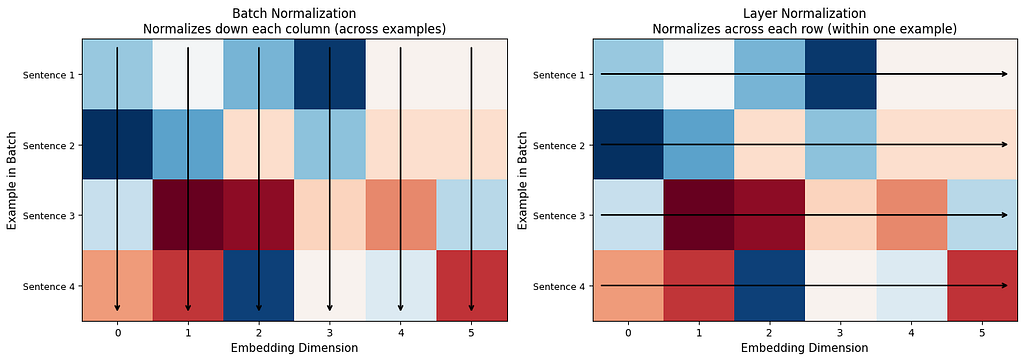
The arrows tell the whole story. Batch Norm looks down columns (comparing across sentences). Layer Norm looks across rows (normalizing within one sentence). For language models, normalizing each word’s embedding on its own terms makes far more sense.
Where Does Layer Norm Go in a Transformer?
Layer Normalization appears in two spots in every Transformer layer, once after attention and once after the feed-forward network. But there are two styles:
Post-Norm (original Transformer): Normalize after the operation.
output = LayerNorm(x + Attention(x))
output = LayerNorm(output + FeedForward(output))
Pre-Norm (modern models like GPT-2 and later): Normalize before the operation.
output = x + Attention(LayerNorm(x))
output = output + FeedForward(LayerNorm(output))
Pre-Norm is what most modern models use because it trains more stably, especially in very deep models with many layers. The numbers stay better behaved from start to finish.
The Residual Connection (Skip Connection)
There is one more piece you may have noticed in the equations above: the x + ... pattern. This is called a residual connection (also known as a skip connection). Instead of replacing the input with the output, the model adds the output to the original input.
Why? Two reasons:
Nothing gets lost. Imagine passing a message through 96 people in a chain. By the end, the original message is probably garbled beyond recognition. But if every person also passes along a photocopy of the original, you always have it available. That is what the residual connection does, it ensures the original embedding survives even after dozens of transformations.
Training works better. During training, the model learns by sending error signals backward through the network (backpropagation). In very deep networks, these signals can fade away before reaching the early layers. The residual connection gives the error signal a direct highway to travel through, bypassing the complex operations.
# Demonstrating the residual connection
np.random.seed(42)
x_original = np.array([1.5, -0.8, 2.1, -1.3, 0.7, -0.2, 1.9, -0.5])

# Simulated attention output
attention_output = np.array([0.3, 0.1, -0.2, 0.4, -0.1, 0.2, -0.3, 0.1])

# Without residual: original information is replaced entirely
without_residual = attention_output
# With residual: original information is preserved and updated
with_residual = x_original + attention_output

print("Original embedding:")
print(f"  {x_original}")
print(f"\nAttention output:")
print(f"  {attention_output}")
print(f"\nWithout residual connection (original information lost):")
print(f"  {without_residual}")
print(f"\nWith residual connection (original information preserved + updated):")
print(f"  {with_residual}")

# How similar is the result to the original?
from numpy.linalg import norm
sim_without = np.dot(x_original, without_residual) / (norm(x_original) * norm(without_residual))
sim_with = np.dot(x_original, with_residual) / (norm(x_original) * norm(with_residual))

print(f"\nSimilarity to original (without residual): {sim_without:.3f}")
print(f"Similarity to original (with residual): {sim_with:.3f}")
Original embedding:
  [ 1.5 -0.8  2.1 -1.3  0.7 -0.2  1.9 -0.5]

Attention output:
  [ 0.3  0.1 -0.2  0.4 -0.1  0.2 -0.3  0.1]

Without residual connection (original information lost):
  [ 0.3  0.1 -0.2  0.4 -0.1  0.2 -0.3  0.1]

With residual connection (original information preserved + updated):
  [ 1.8 -0.7  1.9 -0.9  0.6  0.   1.6 -0.4]

Similarity to original (without residual): -0.530
Similarity to original (with residual): 0.985
With the residual connection, the output is highly similar to the original, the information is almost entirely preserved, with just a small update from attention. Without it, similarity drops sharply and the original signal is gone.
Part 2: Feed-Forward Network: Giving Each Word Its Own Transformation
What Attention Cannot Do
Attention is great at one thing: letting words look at each other and gather context. “Bank” looks at “money” and understands it is in a financial context. But attention is purely a mixing operation, it blends information from different words together.
What attention does not do is transform that gathered information within each word. Once “bank” has collected the context from “money” and “deposited,” something needs to process that combined signal and produce a richer representation. That is the job of the Feed-Forward Network.
Think of it this way: attention is like a student gathering notes from different classmates. The Feed-Forward Network is the student sitting down alone and actually studying those notes, processing, combining, and understanding them.
The Architecture: Expand, Activate, Contract
The feed-forward network is surprisingly simple. It has just two layers with an activation function in between:
FFN(x) = W2 × activation(W1 × x + b1) + b2
Here is what each part does:
W1 (expand): Takes the embedding and makes it bigger, typically 4 times bigger. If the embedding has 768 dimensions (like BERT), W1 expands it to 3072 dimensions.
Activation function: Introduces non-linearity, the ability to learn curved, complex patterns instead of just straight lines. Without this, two linear layers back-to-back would collapse into a single linear layer, and the model would gain nothing.
W2 (contract): Squeezes the expanded representation back down to the original size (768 dimensions).
Why expand and then contract? Think of it like spreading out ingredients on a big table to work with them more easily, then packing the finished dish into a regular-sized container. The bigger workspace lets the model perform more complex operations before compressing the result back to a manageable size.

def feed_forward_network(x, W1, b1, W2, b2, activation='relu'):
    """
    x: input vector (d_model,)
    W1: first linear layer (d_model, d_ff)
    b1: first bias (d_ff,)
    W2: second linear layer (d_ff, d_model)
    b2: second bias (d_model,)
    """
    # Expand: d_model -> d_ff (4x bigger)
    hidden = x @ W1 + b1

    # Activation (non-linearity)
    if activation == 'relu':
        hidden = np.maximum(0, hidden)  # ReLU: if negative, set to zero
    elif activation == 'gelu':
        # GELU: a smoother version used in modern models
        hidden = 0.5 * hidden * (1 + np.tanh(np.sqrt(2/np.pi) * (hidden + 0.044715 * hidden**3)))

    # Contract: d_ff -> d_model (back to original size)
    output = hidden @ W2 + b2

    return output, hidden

# Demonstrate the expand-and-contract pattern
np.random.seed(42)
d_model = 8
d_ff = 32  # 4x expansion

# Initialize weights
W1 = np.random.randn(d_model, d_ff) * 0.1
b1 = np.zeros(d_ff)
W2 = np.random.randn(d_ff, d_model) * 0.1
b2 = np.zeros(d_model)

# Input embedding for one word
x = np.random.randn(d_model)

output, hidden = feed_forward_network(x, W1, b1, W2, b2)

print(f"Input shape: {x.shape} ({d_model} dimensions)")
print(f"Hidden shape: {hidden.shape} ({d_ff} dimensions): 4x expansion")
print(f"Output shape: {output.shape} ({d_model} dimensions): back to original size")
print(f"\nInput: {x.round(3)}")
print(f"Output: {output.round(3)}")
print(f"\nSame shape in, same shape out, but the vector has been transformed.")
Input shape: (8,) (8 dimensions)
Hidden shape: (32,) (32 dimensions): 4x expansion
Output shape: (8,) (8 dimensions): back to original size

Input: [-0.239 -0.908 -0.577  0.755  0.501 -0.978  0.099  0.751]
Output: [-0.     0.017 -0.012  0.065 -0.171 -0.072  0.036 -0.034]

Same shape in, same shape out, but the vector has been transformed.
ReLU vs. GELU: Why the Activation Matters
The activation function is what gives the feed-forward network its power. Without it, stacking two linear layers would just give you one linear layer, mathematically, they would collapse into a single multiplication. The activation introduces non-linearity, which is what lets neural networks learn complex, curved patterns.
ReLU (used in the original Transformer) is the simplest: if the value is positive, keep it. If negative, set it to zero. Like a gate that only lets positive signals through.
GELU (used in BERT, GPT-2, and most modern models) is smoother: instead of a hard cutoff at zero, it gradually scales values down as they approach zero. Small negative values are partially kept instead of being completely zeroed out. This gives the model slightly richer information to learn from.
x_range = np.linspace(-3, 3, 200)
relu = np.maximum(0, x_range)
gelu = 0.5 * x_range * (1 + np.tanh(np.sqrt(2/np.pi) * (x_range + 0.044715 * x_range**3)))

plt.figure(figsize=(10, 5))
plt.plot(x_range, relu, label="ReLU (original Transformer)", linewidth=2.5, color="#e74c3c")
plt.plot(x_range, gelu, label="GELU (modern models)", linewidth=2.5, color="#3498db")
plt.axhline(y=0, color='gray', linewidth=0.5, linestyle='--')
plt.axvline(x=0, color='gray', linewidth=0.5, linestyle='--')
plt.xlabel("Input Value", fontsize=12)
plt.ylabel("Output Value", fontsize=12)
plt.title("ReLU vs. GELU — How Activation Functions Shape the Signal")
plt.legend(fontsize=12)
plt.grid(True, alpha=0.3)
plt.tight_layout()
plt.savefig("relu_vs_gelu.png", dpi=150, bbox_inches="tight")
plt.show()

Notice how ReLU has a sharp corner at zero (everything negative becomes exactly zero), while GELU curves smoothly. That smooth curve means better gradients during training, which adds up across millions of parameters and dozens of layers.
One Critical Detail: Each Word Is Processed Independently
Unlike attention, which mixes information across words, the feed-forward network processes each word on its own. The same weights are used for every word in the sentence, but each word’s vector is transformed separately, no word looks at any other word during this step.
This is by design. Attention handles the “what should I pay attention to?” question. The feed-forward network handles the “given what I gathered, what should I make of it?” question. One is a group activity. The other is individual study.
sentence = ["The", "cat", "sat", "quietly"]

# Shared weights — same for every word
np.random.seed(42)
W1 = np.random.randn(d_model, d_ff) * 0.1
b1 = np.zeros(d_ff)
W2 = np.random.randn(d_ff, d_model) * 0.1
b2 = np.zeros(d_model)

# Each word gets its own embedding (as it comes out of attention)
embeddings = np.random.randn(len(sentence), d_model)

print("Feed-forward applied to each word independently:\n")
for i, word in enumerate(sentence):
    output, _ = feed_forward_network(embeddings[i], W1, b1, W2, b2)
    print(f"  '{word}': input norm = {np.linalg.norm(embeddings[i]):.3f} → output norm = {np.linalg.norm(output):.3f}")

print(f"\nSame weights, different inputs, different outputs.")
print(f"Each word is transformed on its own, based on the context it gathered from attention.")
Feed-forward applied to each word independently:

  'The': input norm = 1.888 → output norm = 0.204
  'cat': input norm = 3.215 → output norm = 0.259
  'sat': input norm = 2.440 → output norm = 0.238
  'quietly': input norm = 2.563 → output norm = 0.179

Same weights, different inputs, different outputs.
Each word is transformed on its own, based on the context it gathered from attention.
How They All Fit Together: One Transformer Layer
Everything from this article and the previous ones combines into a single Transformer layer:
1. Input embeddings (with positional encoding)
      ↓
2. Multi-Head Attention (gather context from other words)
      ↓
3. Add & Layer Norm (stabilize, preserve original signal)
      ↓
4. Feed-Forward Network (transform each word independently)
      ↓
5. Add & Layer Norm (stabilize again)
      ↓
6. Output embeddings (richer, more contextualized)
This block is repeated 12 times in BERT-base, 24 times in GPT-2, and 96 times in GPT-3. Each repetition refines the representation further, early layers capture basic patterns, later layers capture deeper meaning.
def transformer_layer(x, n_heads, d_model, d_ff):
    """One complete Transformer layer (Pre-Norm variant)"""
    gamma = np.ones(d_model)
    beta = np.zeros(d_model)

    W1 = np.random.randn(d_model, d_ff) * 0.02
    b1 = np.zeros(d_ff)
    W2 = np.random.randn(d_ff, d_model) * 0.02
    b2 = np.zeros(d_model)

    # Step 1: Layer Norm → Multi-Head Attention → Add (residual)
    normed = np.array([layer_norm(x[i], gamma, beta)[0] for i in range(len(x))])
    attn_output, _ = multi_head_attention(normed, n_heads, d_model)
    x = x + attn_output

    # Step 2: Layer Norm → Feed-Forward → Add (residual)
    for i in range(len(x)):
        normed_i = layer_norm(x[i], gamma, beta)[0]
        ff_out, _ = feed_forward_network(normed_i, W1, b1, W2, b2, activation='gelu')
        x[i] = x[i] + ff_out

    return x

# Run a sentence through 6 layers and watch how the embedding evolves
np.random.seed(42)
sentence = ["The", "cat", "sat", "quietly"]
d_model = 32
d_ff = 128
n_heads = 4

# Initial embeddings
x = np.random.randn(len(sentence), d_model) * 0.1

print("Tracking 'cat' embedding through 6 layers:\n")
print(f"  Initial: norm = {np.linalg.norm(x[1]):.4f}, first 3 values = {x[1][:3].round(4)}")

for layer_num in range(6):
    x = transformer_layer(x.copy(), n_heads, d_model, d_ff)
    print(f"  Layer {layer_num + 1}: norm = {np.linalg.norm(x[1]):.4f}, first 3 values = {x[1][:3].round(4)}")

print(f"\nThe embedding for 'cat' changes at every layer — each pass adds more context and depth.")
Tracking 'cat' embedding through 6 layers:

  Initial: norm = 0.4971, first 3 values = [-0.0013 -0.1058  0.0823]
  Layer 1: norm = 0.8551, first 3 values = [ 0.0632 -0.1834  0.0447]
  Layer 2: norm = 1.8968, first 3 values = [ 0.2836 -0.1149 -0.1832]
  Layer 3: norm = 2.6312, first 3 values = [ 0.2094 -0.0081  0.2346]
  Layer 4: norm = 3.2021, first 3 values = [ 0.3186 -0.3298  0.369 ]
  Layer 5: norm = 4.3131, first 3 values = [ 0.3818 -0.3652  0.6537]
  Layer 6: norm = 5.0052, first 3 values = [ 0.4674 -0.4816  0.7988]

The embedding for 'cat' changes at every layer — each pass adds more context and depth.
The Key Takeaways
Layer Normalization and the Feed-Forward Network do not get the same attention (pun intended) as the attention mechanism itself. But without them, Transformers would not work.
Layer Normalization is the thermostat of the Transformer, it keeps the numbers at a stable temperature so the model does not overheat or freeze up, no matter how deep it goes. The residual connections make sure that original information is always available, like a safety net that prevents anything from being permanently lost.
The Feed-Forward Network is where each word processes what it has learned. After attention gathers context from the sentence, the feed-forward network transforms each word’s representation individually, expanding it into a larger space, applying a non-linear transformation, and compressing it back down.
Attention decides what information to gather. Layer Norm keeps the signals clean. The Feed-Forward Network decides what to do with what was gathered. Together, they form one Transformer layer — and the power of the Transformer comes from stacking that layer dozens of times.
The Parts of a Transformer Nobody Talks About (But That Make It Work) was originally published in Level Up Coding on Medium, where people are continuing the conversation by highlighting and responding to this story.


