Simulation Functions In Modeldata: How to Craft Purpose-Built Datasets in R Programming

Simulation Functions In Modeldata: Why Purpose-Built Datasets Still Matters for R Programming

The modeldata package now offers simulation tools alongside its curated datasets — and that changes how you can practice data modeling in R.

You have a dataset you need to analyze. Maybe you’re building a classification model for a client, or you’re teaching a workshop on regression techniques. You need practice data that behaves like real-world information — with known relationships between variables, predictable noise levels, and enough structure to test whether your model is actually learning patterns.

You could ask ChatGPT or Claude to generate a CSV with 500 rows. You’d get something back in seconds. The columns would have reasonable names, the values would fall within plausible ranges, and the data would look convincing at first glance.

The problem surfaces when you try to validate your model against that AI-generated data. You have no mathematical guarantee about the relationships embedded in those rows. The correlations between variables may be arbitrary. The noise distribution could be anything. When your model performs well or poorly on AI-generated data, you can’t be sure whether the result reflects your model’s quality or the quirks of how the data was assembled.

The modeldata package addresses this concern directly. In its latest update to version 1.5 (July 2025), the package expanded its simulation toolkit — a set of functions that generate data from documented mathematical equations with known statistical properties. These simulation functions have been quietly evolving since version 1.0, and they now represent the only exported functions in the entire package. The curated datasets are still available through lazy loading, but the simulation toolkit signals where modeldata is heading as a resource for analysts.

I covered the additions to the modeldata package in a previous article. That post is a bit older; since that time the simulation functions became a focus. So for this follow-up I will explain these functions and why they matter for your modeling workflow — especially when AI-generated data feels like the faster option.

The Five Simulation Functions

The modeldata package provides five simulation functions: sim_regression(), sim_classification(), sim_logistic(), sim_multinomial(), and sim_noise(). Each generates data with mathematically defined structures, giving you full control over the data-generating process.

Let’s start with a regression simulation using the newest method added in version 1.5.

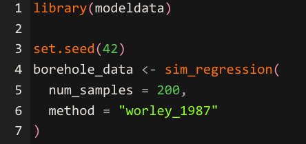
The sim_regression() function accepts a method argument that selects from six documented mathematical models.

"sapp_2014_1" — This methid is the default setting. It uses 20 Gaussian predictors and a prediction equation that mixes linear terms, trigonometric functions (sin), logarithms, squared terms, and interaction effects. This is your go-to for testing whether a model can detect a variety of signal types in the same dataset. If you're comparing a linear regression against a random forest, this method will show you where the linear model breaks down on the nonlinear components.

"sapp_2014_2" — Uses 200 Gaussian predictors where every predictor has the same functional form (log(abs(predictor))). The challenge here is dimensionality. You have a large number of predictors that all contribute equally, which makes this useful for testing variable selection methods and regularization techniques like lasso or elastic net. It reveals whether your approach can handle high-dimensional data where the signal is spread thinly across many columns.

"van_der_laan_2007_1" — Uses 10 binary (Bernoulli) predictors with interaction-heavy relationships. The prediction equation is built entirely from two-way and three-way interaction terms. This is valuable for testing tree-based models and ensemble methods, since the underlying signal depends on combinations of variables rather than individual predictors. A model that only looks at main effects will perform poorly here.

"van_der_laan_2007_2" — Uses 20 Gaussian predictors with a mix of interactions, squared terms, and linear effects. The noise level is high (variance of 16), so the signal-to-noise ratio is deliberately unfavorable. This method is useful for stress-testing your models under noisy conditions and evaluating whether your approach overfits or appropriately regularizes when the data is messy.

"hooker_2004" — Uses 10 predictors with a complex equation involving pi, sqrt, asin, and log transformations. The predictors have different ranges (some standard uniform, others uniform on a narrower interval). This method tests whether your model can handle varied predictor scales and highly nonlinear functional forms. It's particularly useful for evaluating additive models and methods that attempt to decompose predictions into individual feature contributions.

"worley_1987" — This method is the newest addition to modeldata as of version 1.5. It uses a mechanistic engineering model for liquid flow between aquifers. The predictors have physically meaningful names (radius_borehole, transmissibility_upper_aq, etc.) and defined feasible ranges. The error structure is multiplicative rather than additive, meaning the noise scales with the magnitude of the prediction. This is the method to use when you want to practice with data that resembles real-world physical or engineering processes where measurement error grows proportionally with the quantity being measured.

In practical terms, each method isolates a different modeling challenge: mixed signal types (sapp_2014_1), high dimensionality (sapp_2014_2), interaction detection (van_der_laan_2007_1), high noise (van_der_laan_2007_2), nonlinear complexity (hooker_2004), and domain-grounded physical modeling (worley_1987). Choosing the right method depends on which skill you’re trying to sharpen or which model assumption you’re trying to evaluate.

The sim_regression() function with the worley method produces a tibble with physically meaningful predictors like radius_borehole, length_borehole, transmissibility_upper_aq, and conductivity_borehole.

The set.seed() call ensures reproducibility, so anyone running this code will get identical staring point when generating results — a property that AI-generated data cannot guarantee across different sessions or platforms.

Classification Simulations

For classification tasks, sim_classification() generates two-class data with multiple types of predictor effects built into the underlying equation.

The sim_classification() function creates predictors across four categories: two correlated multivariate normal predictors (two_factor_1 and two_factor_2), a set of diminishing linear effects controlled by the num_linear argument, a nonlinear predictor, and Friedman-style interaction terms.

The keep_truth = TRUE argument retains a .truth column containing the error-free outcome value, which allows you to measure how much noise is affecting your model’s performance. The table() call on the class column reveals the class balance, which you can adjust through the intercept parameter to practice handling imbalanced datasets.

Flexible Logistic Simulation

The sim_logistic() function gives you the ability to define your own prediction equation using two correlated predictors.

The visualization produces the image below.

The sim_logistic() function accepts an R formula through the eqn argument, where you specify any mathematical relationship involving predictors A and B. The correlation argument controls the correlation between these two predictors, letting you test how multicollinearity affects your classifier. The formula ~ 2 * A — 3 * B + 1.5 * A * B creates a decision boundary shaped by both main effects and their interaction, producing data where the class separation follows a known mathematical curve.

The ggplot() visualization confirms the boundary pattern, giving you visual verification that the data-generating process matches your expectations.

Multinomial Simulation for Multi-Class Problems

The sim_multinomial() function extends the logistic approach to three-class outcomes, letting you define separate equations for each class.

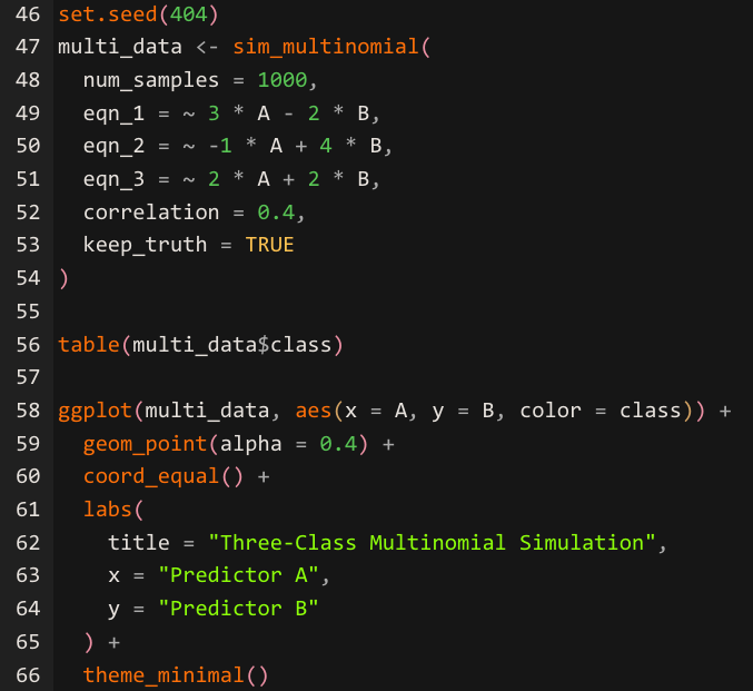
The sim_multinomial() function requires three formula arguments — eqn_1, eqn_2, and eqn_3 — each defining the linear predictor for one of the three classes labeled "one," "two," and "three." The function evaluates and exponentiates each equation, normalizes the resulting values to sum to one across each row, and passes those probabilities to stats::rmultinom() to generate class assignments.

The correlation argument controls the relationship between predictors A and B, just as it does in sim_logistic(). The ggplot() visualization reveals how the three equations create overlapping decision regions, giving you a clear picture of where classification becomes ambiguous — the exact zones where your model's performance will be tested most.

Generating Noise for Benchmarking

The sim_noise() function creates data with no signal — a useful baseline for checking whether your model is finding patterns where none exist.

The sim_noise() function generates multivariate normal variables with mean zero and a covariance structure you control. The cov_type = "toeplitz" argument creates an exponentially decaying correlation pattern between variables — predictors that are closer in index are more correlated than those further apart. The cov_param argument sets the base correlation value. The outcome = "classification" argument adds a class column with randomly assigned labels that have no relationship to the predictors. Running a model on this data provides a sanity check: any model that reports strong performance on pure noise is overfitting.

A Note on the Base Pipe

Version 1.5 also transitioned the package documentation from the magrittr pipe (%>%) to the base R pipe (|>). This means examples throughout the modeldata documentation now use the native pipe introduced in R 4.1. The package itself now requires R 4.1 or later. If you have been using %>% in your scripts, both pipes will continue to work, but new examples from the tidymodels ecosystem will favor the base pipe going forward.

To learn more about the base pipe, you can read my post Iwrote when the base pipe was first introduced.

How to Use The New Pipe in R 4.1

The Pros of Modeldata’s Approach

Modeldata’s simulation functions provide advantages that extend well beyond convenience. The mathematical transparency of each method means you can verify your model against a known ground truth. When sim_regression() generates data using the Sapp (2014) equation, every coefficient, every nonlinear transformation, and every interaction term is documented. You can calculate what the correct prediction should be for any given set of inputs and compare that to what your model produces.

Reproducibility across environments is another advantage. As mentioned earlier, the set.seed() function plays into reproducibility concerns. Setting a seed before calling any simulation function ensures that your colleague in a different office, your student in a different time zone, and your future self revisiting this project six months later will all generate the exact same starting point for simulated data. This consistency makes simulation data ideal for tutorials, homework assignments, and collaborative research where everyone needs to work from identical inputs.

The curated real-world datasets — over 40 of them, covering domains from Alzheimer’s research to Chicago taxi rides to penguin biology — complement the simulations by providing authentic messiness. Real missing values, genuine class imbalances, and actual feature correlations from published research appear throughout these datasets. The combination of clean simulated data and messy real data within a single package gives you a complete practice environment.

The Cons Worth Acknowledging

Modeldata’s simulation functions cover a specific set of mathematical models, and those models may not reflect the data-generating processes in your particular domain. A marketing analyst working with customer behavior data or a supply chain specialist modeling logistics patterns will find that none of the six regression methods closely mirror their real-world scenarios. The simulations are excellent for learning general modeling techniques, and they fall short when you need domain-specific data structures.

The classification options are also limited. The sim_classification() function offers a single method ("caret"), while sim_regression() now provides six methods. Analysts practicing multi-class classification beyond the two-class and three-class options in sim_logistics() and sim_multinomial() will need to look elsewhere for their training data.

AI-generated data fills a different niche. When you need a quick dataset with specific column names, realistic business terminology, and a structure that matches a particular use case — like a customer churn table with 15 demographic and behavioral columns — asking an AI assistant can be faster than configuring a simulation function. The tradeoff is that you lose the mathematical guarantees, but for exploratory prototyping or UI mockups, those guarantees may not matter as much.

What This Means for Your Work

The modeldata package is evolving from a collection of practice datasets into a modeling toolkit. The simulation functions are now the only exported functions in the package, and the addition of the Worley (1987) method in version 1.5 signals that the maintainers are actively expanding this capability.

For analysts and data scientists building models in R, the practical takeaway is to use the right tool for each stage of your workflow. Simulation functions from modeldata give you controlled environments for testing model assumptions, validating pipelines, and benchmarking algorithms. The curated datasets give you realistic complexity for practicing data cleaning and feature engineering. AI-generated data gives you speed when you need a quick prototype or a demo dataset with specific business context.

Understanding where each approach adds value keeps your modeling practice grounded in sound methodology — and that understanding separates an analyst who builds trustworthy models from one who simply runs code.

Updates to the Modeldata library in R Programming