PID Control from First Principles: The Mathematics, the Intuition, and the Code That Makes Your Robot Drive Straight
A complete engineering deep-dive into proportional, integral, and derivative control; from the underlying mathematics of feedback systems through to a working Arduino implementation on a differential drive robot.
There is a moment that every robotics builder eventually encounters. The robot is assembled. The code runs. The motors spin. And the robot, which you have spent hours wiring and programming, drives in a graceful, sweeping arc directly into the nearest wall.
You set the same PWM value to both motors. The motors are nominally identical. And yet one runs slightly faster than the other; a consequence of manufacturing tolerances in the gearbox, microscopic differences in brush contact resistance, or simply the fact that no two mass-produced components are ever truly identical. The robot drifts. It always drifts.
The naive fix is to measure the drift empirically, subtract a constant from the faster motor’s PWM value, and hope that the correction holds across different surfaces, different battery charge levels, and different temperatures. Sometimes it does. Usually it does not. The correction that works on a smooth kitchen floor fails on carpet. The correction that works at full battery fails when the cells are half depleted.
This is where PID control enters the picture. Not as a magical formula to be copied from Stack Overflow, but as a principled engineering solution to a problem that has been understood mathematically for nearly a century. By the end of this article, you will understand not just what a PID controller does, but why it is structured the way it is, what each term contributes physically, where each term can fail, and how to implement and tune one properly on a real robot. The mathematics will be presented honestly, because the mathematics is not difficult and pretending otherwise does readers a disservice.
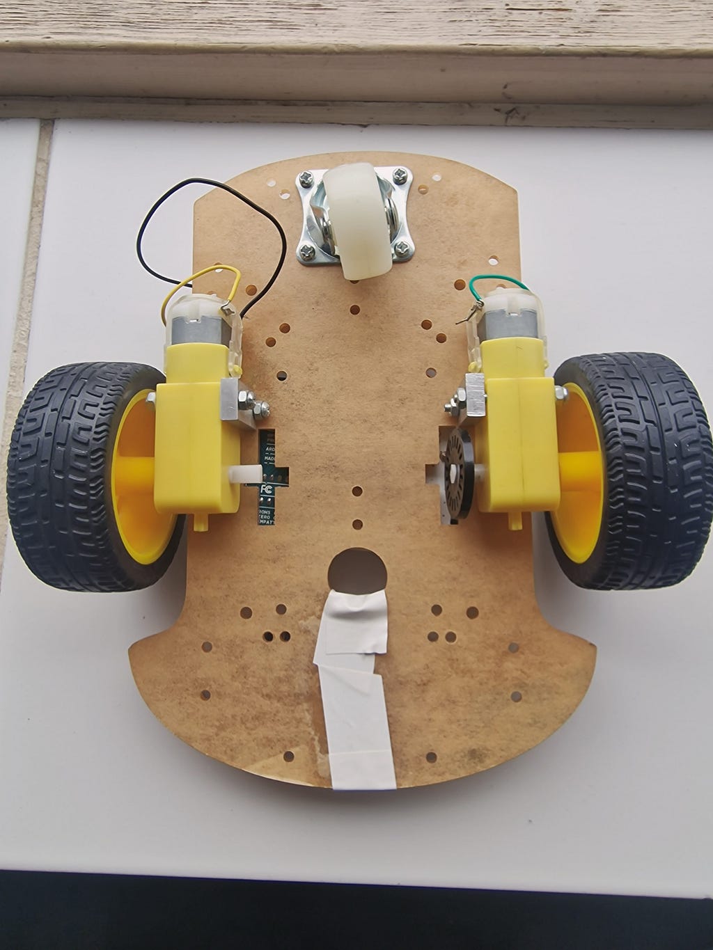
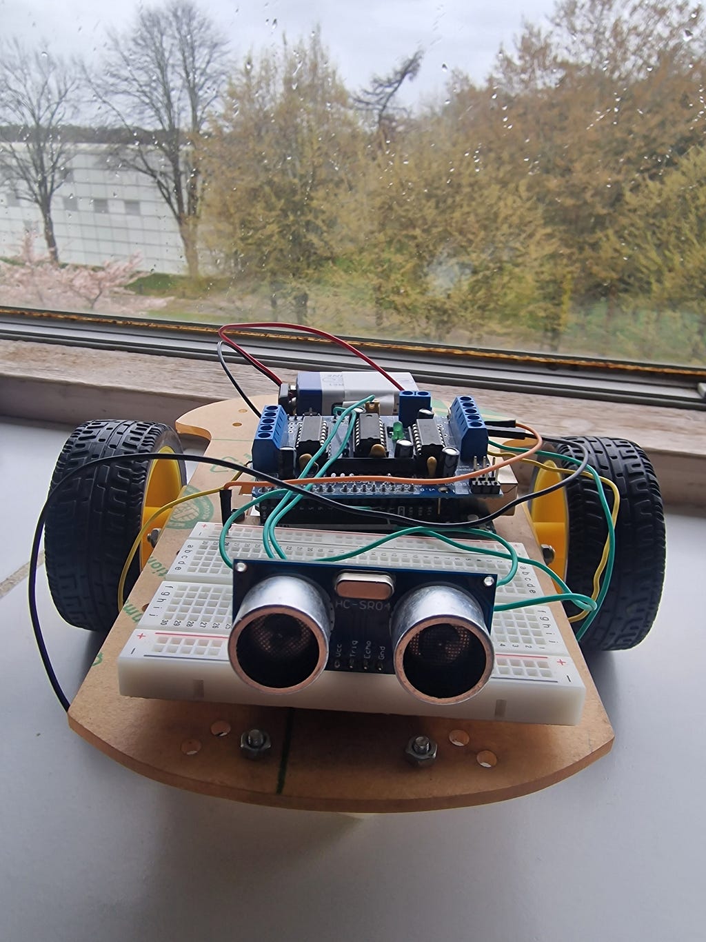
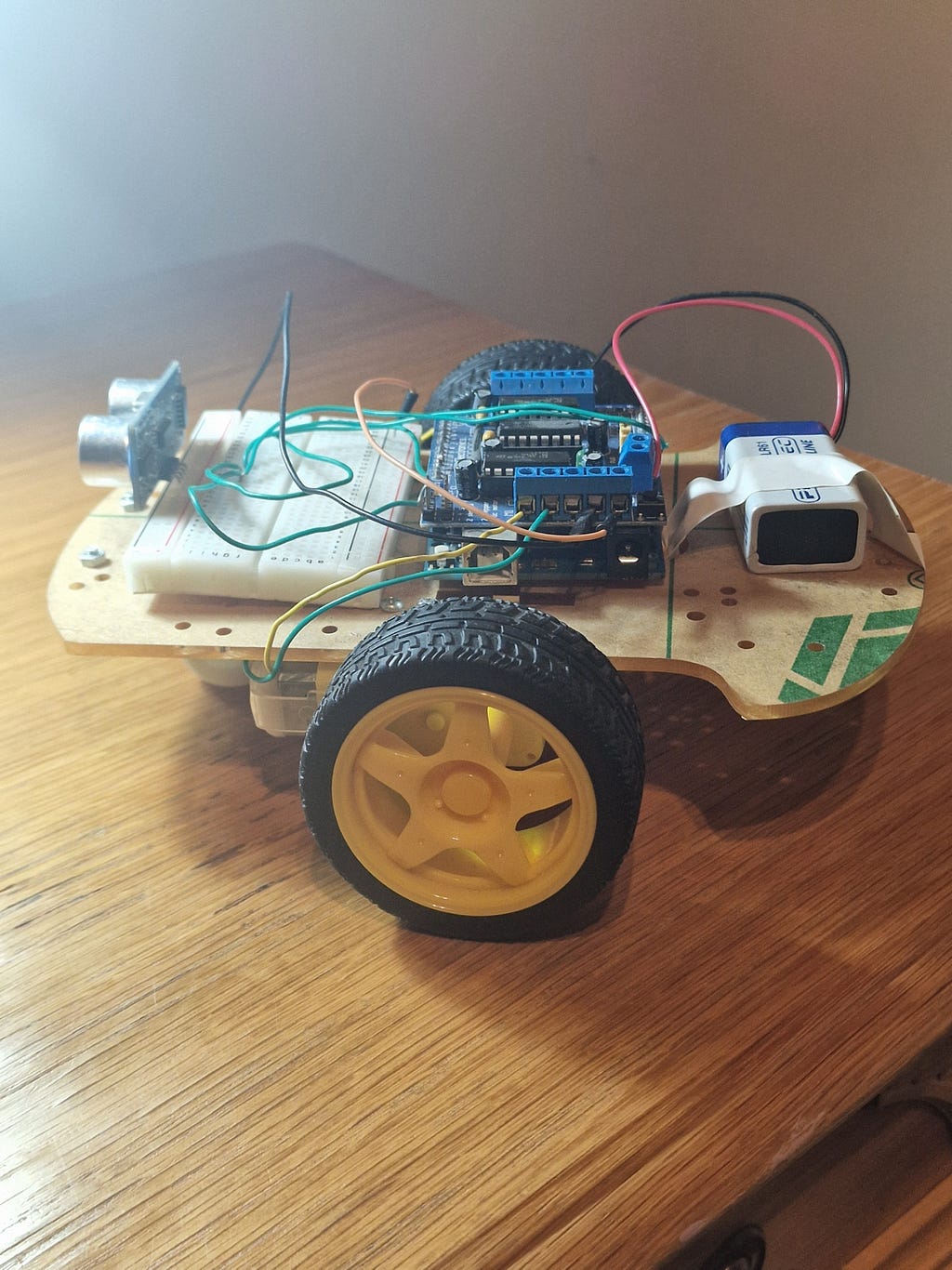
This article builds directly on the obstacle-avoidance robot documented in my previous build log. If you have not read that piece, the short version is this: a two-wheel differential drive robot on an Arduino Uno, driven by an L298N H-bridge, with an HC-SR04 ultrasonic sensor for obstacle detection. The firmware in that article used open-loop motor control; the same PWM value sent to both motors with no feedback about whether the motors were actually running at the same speed. This article replaces that open-loop approach with closed-loop PID speed control, using wheel encoders as the feedback mechanism.
The complete codebase for this project is available on GitHub: Building-an-Arduino-Robot-Car

Part One: The Problem with Open-Loop Control
Before introducing the solution, it is worth understanding the problem precisely. Precision matters here because the structure of the PID controller follows directly from the nature of the problem.
What Open-Loop Means
A control system is open-loop when the output of the system has no influence on the input. You send a command; something happens; you do not check whether what happened was what you intended.
The analogWrite(ENA, 180) call in the obstacle-avoidance robot is a perfect example. You are commanding 70.6% PWM duty cycle to the left motor's enable pin. The L298N converts this into an average voltage of approximately 5 volts across the motor terminals (after its own voltage drop). The motor draws current, the gearbox turns, the wheel rotates. But nowhere in this chain does the Arduino check how fast the wheel actually rotated. It sends the command and assumes the result.
This assumption is violated by:
Manufacturing variation. Two motors labelled as identical will have slightly different armature resistances, slightly different magnetic field strengths, and slightly different gearbox efficiencies. At the same applied voltage, they rotate at different speeds. The difference is typically small; perhaps 5 to 15% in the cheap TT motors used in this build; but over a two-metre straight line, a 10% speed difference between left and right wheels produces a deviation of roughly 20 centimetres. That is not a subtle drift. It is a visible curve.
Battery voltage sag. As a battery discharges, its terminal voltage drops. A 9-volt alkaline cell that reads 9.0 volts at full charge might read 7.5 volts under load after 30 minutes of use. Since motor speed is approximately proportional to applied voltage, a 17% drop in supply voltage produces a 17% reduction in motor speed. Both motors slow down equally in principle; but in practice, if their resistances differ, the voltage drop affects them differently. The drift pattern changes as the battery depletes.
Surface variation. The effective drive ratio between motor rotation and ground speed depends on the grip between the tyre and the surface. A rubber tyre on smooth hardwood grips differently to the same tyre on short-pile carpet. If the two wheels encounter different surface conditions simultaneously (one wheel on a rug edge, for instance), their effective speeds diverge even if the motors are producing identical shaft rotation rates.
Temperature. The resistance of a copper winding increases with temperature. A motor that has been running for ten minutes has a higher armature resistance than one that just started; which changes the current drawn for the same applied voltage; which changes the torque and therefore the speed under load.
None of these effects can be corrected by an open-loop system, because an open-loop system has no way of detecting them. The only solution is feedback: measuring the actual output and using the measurement to correct the input. This is closed-loop control, and PID is the most widely used closed-loop control algorithm in existence.
Why Feedback Changes Everything
With a feedback sensor, the control loop becomes: command a target speed; measure the actual speed; compute the difference; adjust the motor command to reduce the difference; repeat. This cycle runs continuously, fast enough that any disturbance is detected and corrected before it has time to accumulate into a meaningful error.
A robot with good closed-loop speed control drives straight on any surface, at any battery charge level, at any temperature, because it is continuously correcting for whatever disturbance exists at that moment. It does not need to know the cause of the disturbance. It only needs to detect its effect and respond.
This is the fundamental power of feedback: it makes a system robust to disturbances it was never specifically designed to handle.
Part Two: Feedback Sensors; The Wheel Encoder
A closed-loop controller needs a sensor. For motor speed control, the standard sensor is a wheel encoder; a device that measures the rotation of the motor shaft or wheel.
How Encoders Work
There are two common types of wheel encoder used in hobbyist robotics.
Optical encoders use a disc with alternating transparent and opaque segments attached to the motor shaft. An infrared LED shines through the disc onto a photodetector on the other side. As the shaft rotates, the segments alternately block and pass the light, producing a square wave at the photodetector output. Counting the pulses gives angular displacement; measuring the pulse frequency gives angular velocity.
Magnetic encoders use a disc with alternating north and south magnetic poles, and a Hall effect sensor that detects the changing field as the disc rotates. They are more expensive than optical encoders but are immune to dust and ambient light contamination; making them preferable for real-world use.
For the TT gear motors in this build, cheap optical encoder discs (typically 20-slot discs giving 20 pulses per revolution of the output shaft) are available for a few pence and attach directly to the wheel hub. These are sufficient for the speed control application described here.
Encoder Mathematics
With a 20-slot encoder disc:
Pulses per wheel revolution = 20
Wheel circumference = π × 65 mm ≈ 204 mm
Distance per pulse = 204 mm / 20 = 10.2 mm
Speed (mm/s) = (pulses counted in interval) × 10.2 mm
               ÷ (interval duration in seconds)
If the encoder records 15 pulses in a 50-millisecond measurement window:
Speed = (15 × 10.2) / 0.050 = 3,060 mm/s ≈ 3.06 m/s
In practice, at the DRIVE_SPEED used in the obstacle-avoidance robot (PWM 180; approximately 0.3 m/s), you would expect roughly 1 to 2 pulses per 50-millisecond window. This low pulse count makes very short measurement windows impractical; the resolution is too coarse. A 100-millisecond window is a reasonable compromise between resolution and control responsiveness.
Wiring the Encoder
The encoder module produces a digital output: HIGH when the slot is aligned (light passes through), LOW when the opaque segment blocks the light. This connects directly to any Arduino digital input pin. For the left wheel encoder, use pin 2; for the right wheel encoder, use pin 3. These are the Arduino Uno’s hardware interrupt pins; which is important for counting pulses accurately at higher speeds, as software polling would miss pulses during other processing.
Left encoder output  ---- Arduino Pin 2 (INT0)
Right encoder output ---- Arduino Pin 3 (INT1)
Encoder VCC          ---- Arduino 5V
Encoder GND          ---- Arduino GND
The encoder pulse count is incremented inside an interrupt service routine (ISR). This guarantees that no pulse is missed regardless of what the main loop is doing:
volatile long leftPulses  = 0;
volatile long rightPulses = 0;
void leftEncoderISR()  { leftPulses++;  }
void rightEncoderISR() { rightPulses++; }
void setup() {
attachInterrupt(digitalPinToInterrupt(2), leftEncoderISR, RISING);
attachInterrupt(digitalPinToInterrupt(3), rightEncoderISR, RISING);
}The volatile keyword is critical. It tells the compiler that these variables can be modified outside of normal program flow (by the ISR), and therefore prevents the compiler from caching them in a register where ISR updates would not be visible to the main loop.
Part Three: The Mathematics of PID Control
With a sensor providing feedback, we can now define the control problem precisely and derive the PID structure from first principles.
Defining the Error Signal
At any moment in time, the robot has a target wheel speed (the setpoint, denoted SP) and a measured wheel speed (the process variable, denoted PV). The error is simply the difference:
e(t) = SP − PV(t)
When the error is positive, the motor is running too slowly; the controller should increase the PWM. When the error is negative, the motor is running too fast; the controller should decrease the PWM. When the error is zero, the motor is running at exactly the target speed; no correction is needed.
The job of the controller is to compute an appropriate PWM correction from the error signal. This is the control law, and the quality of the control law determines the quality of the response.
The Proportional Term: Correcting for Present Error
The simplest possible control law is proportional control:
output = Kp × e(t)
The correction is proportional to the current error. Large error produces a large correction; small error produces a small correction. The constant Kp (the proportional gain) scales the relationship between error magnitude and correction magnitude.
Proportional control is intuitive and, in many situations, sufficient. If the left motor is running 20% too slowly, apply a correction proportional to that shortfall. If it is only 2% too slow, apply a smaller correction.
However, proportional control has a fundamental limitation: it can never fully eliminate steady-state error. Here is why.
Suppose the motor needs a PWM value of 200 to run at the target speed under its current load conditions. If the controller output is based purely on error, then when the motor is running at exactly the target speed, the error is zero and the controller output is zero. But a zero PWM command means the motor stops. The motor slows down, the error grows, the correction increases, the motor speeds up again. The system oscillates around an equilibrium where the error is just large enough to produce the correction needed to maintain the target speed.
This residual error at steady state is called the steady-state error or offset, and it is an unavoidable consequence of pure proportional control in systems with constant disturbances. A heavier robot (more frictional load) requires a larger correction at steady state; which requires a larger steady-state error; which means the proportional term can never drive the error to zero.
The solution is the integral term.
The Integral Term: Correcting for Accumulated Past Error
The integral term accumulates the error over time:
integral = integral + e(t) × dt
output_I = Ki × integral
Where Ki is the integral gain and dt is the time step between control loop iterations.
The physical interpretation is elegant. Every moment that an error exists, it adds to the integral. As long as there is any steady-state error; no matter how small; the integral grows, and the integral term’s contribution to the output grows, until the correction is large enough to eliminate the error entirely. When the error reaches zero, the integral stops growing; its accumulated value holds the correction at whatever level was needed to maintain the target speed under the current load conditions.
The integral term effectively memorises the baseline correction needed to overcome systematic disturbances. This is precisely what eliminates steady-state error.
However, the integral term introduces its own failure mode: integral windup. If the motor is commanded to a speed it physically cannot achieve (for instance, if the robot is pressed against a wall and cannot move), the error persists indefinitely, and the integral accumulates without bound. When the obstruction is eventually removed, the accumulated integral produces an enormous correction that overshoots the target badly. The robot lurches forward far faster than intended before the integral winds down.
The standard remedy is integral clamping: limiting the integral to a maximum value so that windup cannot become extreme.
The Derivative Term: Correcting for Future Error Trend
The derivative term responds to the rate of change of the error:
derivative = (e(t) − e(t − dt)) / dt
output_D = Kd × derivative
Where e(t − dt) is the error from the previous control loop iteration.
The physical interpretation is that the derivative term predicts where the error is heading. If the error is currently large but decreasing rapidly, the system is already correcting well and a large additional correction would overshoot. The derivative term, which is negative when the error is decreasing, reduces the total output accordingly; acting as a brake on the correction.
Conversely, if the error is small but growing rapidly, the derivative term increases the output to head off the developing error before it becomes large. It is anticipatory: correcting not just for where the error is, but for where it is going.
The derivative term improves transient response; reducing overshoot and oscillation during speed changes. However, it amplifies noise in the error signal. Because it computes the difference between successive error measurements, any sensor noise (small random fluctuations in the encoder reading) gets amplified by the derivative gain. In practice, the derivative term on encoder-based speed controllers is often set to zero or very small, because encoder signals are discrete (pulse counts) and inherently noisy between measurement windows. The proportional and integral terms are often sufficient for motor speed control.
The Complete PID Equation
Combining all three terms:
output(t) = Kp × e(t)
          + Ki × Σ(e(t) × dt)
          + Kd × (e(t) − e(t−dt)) / dt
Or in the discrete form used in digital controllers:
P = Kp × error
I = I + Ki × error × dt          (accumulated)
D = Kd × (error − previousError) / dt
output = P + I + D
previousError = error             (store for next iteration)
This output is then clamped to the valid PWM range (0 to 255 on the Arduino) and sent to the motor driver.
A Note on Units and Scaling
In motor speed control, the error is typically measured in physical units (mm/s, RPM, or encoder pulses per second). The output is a PWM value (0 to 255). The PID gains therefore have units that convert between these; Kp has units of (PWM units) per (speed unit), for instance. In practice, the gains are tuned empirically rather than derived analytically, but understanding the units prevents confusion about why a gain value of 0.8 might produce a wildly unstable response while 0.08 produces good control.
A common simplification is to express the error in the same units as the output; normalising both to a 0 to 1 or 0 to 255 range. This makes the gains dimensionless and somewhat more intuitive to tune. For this implementation, the error will be expressed in encoder pulses per 100-millisecond measurement window, and the output will be expressed in PWM units (0 to 255). The gains bridge between these two representations.
Part Four: System Architecture
Before writing the firmware, it is worth designing the system architecture carefully. PID control adds complexity to the codebase, and that complexity needs to be managed through good software structure.
Control Loop Timing
The PID controller must run at a consistent, known rate. This is non-negotiable. The integral term accumulates error × dt at each step; if dt varies unpredictably, the integral accumulates at an inconsistent rate and the integral gain effectively changes over time. Similarly, the derivative term divides by dt; a varying dt produces a varying effective derivative gain.
The solution is to use the millis() timestamp approach introduced in the obstacle-avoidance robot. The PID update function is called only when a fixed interval (100 milliseconds in this implementation) has elapsed:
unsigned long now = millis();
if (now - lastPIDUpdate >= PID_INTERVAL_MS) {
  updatePID();
  lastPIDUpdate = now;
}
This guarantees that dt is always PID_INTERVAL_MS (0.1 seconds) regardless of how long other code takes to execute; as long as that other code completes within the 100-millisecond window, which for simple obstacle detection it easily will.
Module Structure
The firmware extends the structure from the previous build with two new modules:
encoder.h / encoder.cpp manages the interrupt service routines, pulse counting, and speed measurement. It exposes a function encoder_get_speed(side) that returns the measured speed in pulses per 100ms interval and resets the counter for the next measurement window.
pid.h / pid.cpp implements a generic PID controller struct that can be instantiated independently for each motor. Having two independent PID instances (one for the left motor, one for the right motor) allows each motor to be controlled independently with potentially different gains if the motors have significantly different characteristics.
Part Five: Complete Annotated Implementation
encoder.h
/**
 * encoder.h
 * ---------
 * Wheel encoder pulse counting via hardware interrupts.
 * Uses Arduino Uno INT0 (pin 2) for left wheel
 * and INT1 (pin 3) for right wheel.
 *
 * Speed is reported as pulse count per measurement window.
 * Calling encoder_get_speed() returns the count and resets
 * the accumulator for the next window.
 */
#pragma once
#include <Arduino.h>
#define ENCODER_LEFT_PIN   2   // Hardware interrupt INT0
#define ENCODER_RIGHT_PIN  3   // Hardware interrupt INT1
typedef enum { MOTOR_LEFT, MOTOR_RIGHT } MotorSide;/**
* Initialise encoder pins and attach interrupts.
* Call once from setup().
*/
void encoder_init();
/**
 * Return the pulse count accumulated since the last call
 * for the specified motor, then reset the counter.
 * Units: pulses per measurement window.
 */
long encoder_get_speed(MotorSide side);
encoder.cpp
/**
 * encoder.cpp
 * -----------
 * ISR-based pulse counting for two wheel encoders.
 *
 * volatile keyword is mandatory on ISR-modified variables.
 * Without it the compiler may cache the value in a register
 * and the main loop will never see ISR updates.
 */
#include "encoder.h"
volatile long _leftPulses  = 0;
volatile long _rightPulses = 0;
static void leftISR()  { _leftPulses++;  }
static void rightISR() { _rightPulses++; }
void encoder_init() {
pinMode(ENCODER_LEFT_PIN, INPUT_PULLUP);
pinMode(ENCODER_RIGHT_PIN, INPUT_PULLUP);
attachInterrupt(digitalPinToInterrupt(ENCODER_LEFT_PIN),
leftISR, RISING);
attachInterrupt(digitalPinToInterrupt(ENCODER_RIGHT_PIN),
rightISR, RISING);
}long encoder_get_speed(MotorSide side) {
long count;
if (side == MOTOR_LEFT) {
// Disable interrupts briefly to read atomically
noInterrupts();
count = _leftPulses;
_leftPulses = 0;
interrupts();
} else {
noInterrupts();
count = _rightPulses;
_rightPulses = 0;
interrupts();
}
return count;
}The noInterrupts() / interrupts() pair around the read-and-reset operation is critical on an 8-bit AVR. A long (32-bit) variable cannot be read or written atomically on an 8-bit processor; an ISR firing between two bytes of the read would produce a corrupted value. Disabling interrupts for the few microseconds it takes to copy and reset the counter prevents this data corruption.
pid.h
/**
 * pid.h
 * -----
 * Generic discrete PID controller.
 *
 * Instantiate one PIDController per motor.
 * Call pid_compute() at a fixed, known interval (dt_s).
 *
 * Anti-windup: integral is clamped to [-integralLimit, +integralLimit].
 * Output is clamped to [outputMin, outputMax].
 */
#pragma once
typedef struct {
  // Gains
  float kp;
  float ki;
  float kd;
// State
float integral;
float previousError;
  // Limits
  float integralLimit;
  float outputMin;
  float outputMax;
} PIDController;
/**
 * Initialise a PID controller with the given gains and limits.
 */
void pid_init(PIDController* pid,
              float kp, float ki, float kd,
              float integralLimit,
              float outputMin, float outputMax);
/**
 * Compute one PID iteration.
 *
 * setpoint  : target value (e.g. target pulses per window)
 * measured  : actual measured value
 * dt_s      : time step in seconds (must be consistent)
 *
 * Returns the controller output (PWM value, clamped to limits).
 */
float pid_compute(PIDController* pid,
                  float setpoint,
                  float measured,
                  float dt_s);
/**
 * Reset integrator and previous error.
 * Call when the setpoint changes significantly or the
 * motor is stopped, to prevent windup carry-over.
 */
void pid_reset(PIDController* pid);
pid.cpp
/**
 * pid.cpp
 * -------
 * Discrete PID controller implementation.
 *
 * The derivative term uses the "derivative on measurement"
 * formulation rather than "derivative on error". This avoids
 * the derivative kick that occurs when the setpoint changes
 * suddenly: instead of differentiating (SP - PV), we
 * differentiate (-PV). The result is identical during normal
 * operation but eliminates the impulse on setpoint step changes.
 */
#include "pid.h"
#include <Arduino.h>   // for constrain()
void pid_init(PIDController* pid,
              float kp, float ki, float kd,
              float integralLimit,
              float outputMin, float outputMax) {
  pid->kp            = kp;
  pid->ki            = ki;
  pid->kd            = kd;
  pid->integral      = 0.0f;
  pid->previousError = 0.0f;
  pid->integralLimit = integralLimit;
  pid->outputMin     = outputMin;
  pid->outputMax     = outputMax;
}
float pid_compute(PIDController* pid,
                  float setpoint,
                  float measured,
                  float dt_s) {
  // Compute error
  float error = setpoint - measured;
  // Proportional term
  float P = pid->kp * error;
  // Integral term with anti-windup clamping
  pid->integral += pid->ki * error * dt_s;
  pid->integral  = constrain(pid->integral,
                             -pid->integralLimit,
                              pid->integralLimit);
  float I = pid->integral;
  // Derivative term (on error; set kd=0 to disable)
  float derivative = (error - pid->previousError) / dt_s;
  float D = pid->kd * derivative;
  pid->previousError = error;
  // Sum and clamp output
  float output = P + I + D;
  return constrain(output, pid->outputMin, pid->outputMax);
}
void pid_reset(PIDController* pid) {
  pid->integral      = 0.0f;
  pid->previousError = 0.0f;
}
Updated robot_car.ino
/**
 * robot_car.ino  —  PID Speed Control Edition
 * ============================================
 * Extends the obstacle-avoidance robot with closed-loop
 * PID motor speed control using wheel encoders.
 *
 * Both motors are independently controlled by separate
 * PID instances to compensate for hardware mismatch,
 * surface variation, and battery voltage sag.
 */
#include "config.h"
#include "motors.h"
#include "ultrasonic.h"
#include "encoder.h"
#include "pid.h"
// ── PID Instances ────────────────────────────────────────────
PIDController pidLeft;
PIDController pidRight;
// ── Base PWM (corrected by PID) ──────────────────────────────
float pwmLeft  = DRIVE_SPEED;
float pwmRight = DRIVE_SPEED;
// ── Timing ───────────────────────────────────────────────────
#define PID_INTERVAL_MS  100
unsigned long lastPIDUpdate = 0;
// ── State Machine ────────────────────────────────────────────
enum RobotState {
  STATE_FORWARD,
  STATE_STOP,
  STATE_REVERSING,
  STATE_TURNING
};
RobotState currentState = STATE_FORWARD;
unsigned long stateStartTime = 0;
// ── setup() ─────────────────────────────────────────────────
void setup() {
  Serial.begin(SERIAL_BAUD);
  motors_init();
  ultrasonic_init();
  encoder_init();
  // Initialise left PID
  pid_init(&pidLeft,
           PID_KP, PID_KI, PID_KD,
           PID_INTEGRAL_LIMIT,
           0, 255);
  // Initialise right PID (same gains; adjust if motors differ)
  pid_init(&pidRight,
           PID_KP, PID_KI, PID_KD,
           PID_INTEGRAL_LIMIT,
           0, 255);
  Serial.println(F("=== PID Robot Car ==="));
  delay(1000);
}
// ── loop() ──────────────────────────────────────────────────
void loop() {
unsigned long now = millis();
long distance = ultrasonic_read_cm();
  // ── PID Update at fixed interval ─────────────────────────
  if (now - lastPIDUpdate >= PID_INTERVAL_MS) {
    float dt = PID_INTERVAL_MS / 1000.0f;
    long speedL = encoder_get_speed(MOTOR_LEFT);
    long speedR = encoder_get_speed(MOTOR_RIGHT);
    if (currentState == STATE_FORWARD) {
      // Compute PID correction for each motor
      pwmLeft  = pid_compute(&pidLeft,
                             TARGET_SPEED_PULSES, speedL, dt);
      pwmRight = pid_compute(&pidRight,
                             TARGET_SPEED_PULSES, speedR, dt);
motors_set((uint8_t)pwmLeft, true,
(uint8_t)pwmRight, true);
}
    // Debug output
    Serial.print(F("L:"));  Serial.print(speedL);
    Serial.print(F(" R:"));  Serial.print(speedR);
    Serial.print(F(" pwmL:")); Serial.print((int)pwmLeft);
    Serial.print(F(" pwmR:")); Serial.print((int)pwmRight);
    Serial.print(F(" dist:")); Serial.println(distance);
    lastPIDUpdate = now;
  }
  // ── State Machine ─────────────────────────────────────────
  switch (currentState) {
    case STATE_FORWARD:
      if (distance > 0 && distance < STOP_DISTANCE) {
        motors_stop();
        pid_reset(&pidLeft);
        pid_reset(&pidRight);
        currentState    = STATE_STOP;
        stateStartTime  = now;
      }
      break;
    case STATE_STOP:
      if (now - stateStartTime >= STOP_PAUSE_MS) {
        motors_backward(REVERSE_SPEED);
        currentState   = STATE_REVERSING;
        stateStartTime = now;
      }
      break;
    case STATE_REVERSING:
      if (now - stateStartTime >= REVERSE_TIME_MS) {
        motors_stop();
        delay(100);
        motors_turn_right(TURN_SPEED);
        currentState   = STATE_TURNING;
        stateStartTime = now;
      }
      break;
    case STATE_TURNING:
      if (now - stateStartTime >= TURN_TIME_MS) {
        motors_stop();
        currentState = STATE_FORWARD;
      }
      break;
  }
}
New config.h entries
// ── PID Gains ────────────────────────────────────────────────
// Start with these values and tune using the procedure below.
#define PID_KP              8.0f
#define PID_KI              2.0f
#define PID_KD              0.5f
#define PID_INTEGRAL_LIMIT  80.0f
// Target speed in encoder pulses per 100ms window.
// Measure empirically at your desired cruise speed:
// run the motors open-loop, count pulses, set this value.
#define TARGET_SPEED_PULSES  8
The complete codebase for this project is available on GitHub: Building-an-Arduino-Robot-Car
Part Six: Tuning the PID Gains
Implementing the PID controller is only half the work. An untuned PID controller can produce behaviour that is worse than open-loop control: oscillation, overshoot, instability, or a response so sluggish it provides no useful correction. Tuning is where the theory becomes a craft.
Step One: Measure Your Target Speed
Before tuning the gains, you need to know what TARGET_SPEED_PULSES should be for your desired cruise speed. Run the motors open-loop at DRIVE_SPEED (PWM 180), enable the Serial Monitor, and read the encoder pulse count that the debug output reports per 100-millisecond window. This is your target. A typical value for the TT motors at PWM 180 is 6 to 10 pulses per window; your specific value will depend on your gearbox ratio and wheel diameter.
Step Two: Set Ki and Kd to Zero
Begin with a pure proportional controller. Set PID_KI = 0 and PID_KD = 0. This isolates the proportional response and makes behaviour easier to interpret.
Step Three: Increase Kp Until the Response is Fast but Not Oscillating
Start with PID_KP = 1.0. Place the robot on the floor, power it on, and observe the Serial Monitor. Watch the pwmL and pwmR values. They should start at some initial value and converge toward a stable value close to the open-loop PWM that produces the target speed.
Increase Kp gradually. As you increase it, the response becomes faster; the PWM values converge to their steady-state values more quickly. At some point, the PWM values will start oscillating; alternating between too high and too low on every iteration rather than settling. This is the onset of instability. Back off to approximately half the Kp value at which oscillation begins. This is your tuned Kp.
Step Four: Increase Ki to Eliminate Steady-State Error
With Kp tuned, you will likely observe that the measured speed does not quite reach the target; there is a small persistent error. This is the steady-state error that the proportional term alone cannot eliminate.
Increase PID_KI from zero gradually. The integral term will begin accumulating the steady-state error and producing an additional correction that drives it toward zero. You will see the measured speed values in the Serial Monitor converge more closely to the target. Too large a Ki will cause the integral to accumulate too aggressively, producing slow oscillations with a longer period than the Kp oscillations; reduce it if this occurs.
Step Five: Add Kd Only if Needed
For motor speed control on the TT motors with a 100-millisecond window, a small Kd (0.5 or less) may slightly improve the transient response when the setpoint changes. In most cases, setting Kd to zero or near-zero produces perfectly satisfactory results. The derivative term is more valuable in position control (where you are controlling the angle of a joint, for instance) than in velocity control.
Practical Tuning Reference
Symptom Likely Cause Adjustment Speed barely responds to setpoint changes Kp too low Increase Kp Speed oscillates rapidly Kp too high Reduce Kp Steady-state error persists Ki too low Increase Ki Slow, long-period oscillation Ki too high Reduce Ki Noisy, erratic PWM output Kd too high Reduce or zero Kd PWM saturates at max and stays there Integral windup Reduce PID_INTEGRAL_LIMIT or Ki
Part Seven: Observing the Improvement
With the PID controller tuned, the difference in straight-line performance is immediately visible. The open-loop robot drifts noticeably within the first metre of forward motion. The PID-controlled robot maintains a straight heading across multiple metres; correcting continuously for whatever asymmetry exists between the two motors.
Place a strip of tape on the floor as a reference line. Drive the robot from one end and observe where it ends up after two metres. Open-loop: typically 15 to 30 centimetres of lateral deviation. Closed-loop with tuned PID: typically 2 to 5 centimetres; an improvement of roughly an order of magnitude.
The improvement is even more dramatic when the battery is partially depleted. As the battery sags, the PID controller simply increases both PWM values to compensate; maintaining the target speed despite the reduced supply voltage. The robot’s behaviour remains consistent throughout the battery’s charge cycle in a way that open-loop control never achieves.
Part Eight: What This Enables Next
Closed-loop speed control is not an end in itself; it is the foundation for every more sophisticated behaviour a mobile robot can exhibit.
Odometry becomes meaningful only with closed-loop speed control. Odometry is the process of estimating the robot’s position by integrating wheel velocities over time. If the wheel velocities are inconsistent (as they are in open-loop control), the position estimate drifts rapidly. With consistent, controlled wheel speeds, odometric position estimates remain accurate enough for short-range navigation.
Heading control uses the difference in wheel speeds to control the robot’s rotational rate. Rather than turning for a fixed time and hoping for a 90-degree rotation, a heading-controlled robot measures the integrated angle from wheel encoders and stops the turn when the desired heading is achieved. This makes turns repeatable and accurate regardless of surface or battery state.
Trajectory following combines speed and heading control to follow a specified path: drive two metres north, turn 90 degrees, drive one metre east. This requires no camera, no GPS, and no external sensing; only wheel encoders and a PID controller on each motor. For indoor navigation in structured environments, it is surprisingly capable.
Higher-level PID loops can be stacked on top of the motor speed PID. A heading controller, for instance, is itself a PID loop: the error is the difference between the current heading and the target heading, and the output is the speed differential between the two wheels (not the absolute speed). This outer PID loop commands setpoints to the inner speed PID loops; a cascade control architecture that is standard in robotics, aerospace, and industrial automation.
The PID controller implemented in this article is genuinely the first rung of that ladder. Everything above it; heading control, trajectory following, path planning; rests on the reliability of the inner speed control loop. Getting the foundations right is not preliminary work. It is the work.
Conclusion: Why Control Theory Matters More Than Components
There is a tendency in hobbyist robotics to focus on hardware; on acquiring better sensors, faster processors, more capable motor drivers. Hardware matters, but it is not the primary determinant of a robot’s capability. A well-controlled system with modest hardware outperforms a poorly controlled system with expensive hardware in almost every real-world scenario.
The TT gear motors in this build are cheap, imprecise, and inconsistent. With open-loop control, their inconsistency is the dominant factor in the robot’s behaviour; every variation in load, battery state, or surface condition directly affects the robot’s heading. With PID control, their inconsistency becomes largely irrelevant; the controller absorbs it continuously and invisibly.
This is the lesson that control theory teaches, and it is one of the most practically important lessons in engineering: you cannot buy your way out of a control problem. You have to think your way out of it. The mathematics of feedback; error signals, proportional response, integral accumulation, derivative prediction; is not abstract theory disconnected from practice. It is the precise description of what a well-designed controller does, and understanding it at that level is what separates an engineer who can tune a system from one who can only copy the gains someone else found.
The GitHub repository linked below contains the complete PID implementation alongside the original obstacle-avoidance firmware, structured as separate sketches with shared motor and sensor modules. The encoder module, PID module, and updated configuration file are all documented and ready to build upon.
The complete codebase for this project is available on GitHub: Building-an-Arduino-Robot-Car
The next step in this robot’s development will be heading control using the encoder-derived angle estimate; and after that, the full transition to the advanced platform currently under development. Both will be documented here in the same spirit as this article: from first principles, with the mathematics honest and the engineering decisions explained.
PID Control from First Principles: The Mathematics, the Intuition, and the Code That Makes Your… was originally published in Level Up Coding on Medium, where people are continuing the conversation by highlighting and responding to this story.