How to shrink your ML model 9× and make it 6× faster

From zero to production-ready: pruning, quantization, and knowledge distillation explained with working code.

You spent three weeks training a model.

Accuracy: 94%. Loss curve: beautiful. You’re proud of it.

Then you try to deploy it.

The inference server chokes. The Docker container crashes past memory limits. The API takes 4 seconds to respond. Your users leave.

This is the gap nobody talks about in ML tutorials , the space between model trained and model deployed. Most courses end right at the moment the real engineering begins.

I’ve been competing on Kaggle and building ML systems for production deployments, and this problem comes up constantly. It’s the reason most ML projects never make it past a notebook.

This article closes that gap entirely. By the time you finish reading, you’ll understand how to shrink a 400MB model down to under 45MB, cut inference time by 6×, and lose almost none of the accuracy you worked so hard for.

We’ll cover three core techniques that every production ML engineer uses:

1. Pruning — cutting the parts of your network that don’t contribute
2. Quantization — storing weights in fewer bits
3. Knowledge Distillation — training a small model to think like a big one

For each one: intuition first, math second, code third, with every line explained. Whether you’re reading about this for the first time or you’ve tried these techniques before and hit walls, this guide is written for you.

Why Do Models Get So Big?

Before we fix the problem, we need to understand why it exists.

When you train a neural network, the only thing the training process optimizes for is accuracy on your validation set. Nothing about that objective cares about:

• How many parameters your model has
• How much RAM it needs at inference time
• How fast it runs on a server

So naturally, models balloon. Engineers add more layers, more neurons, more capacity , because more parameters almost always means better accuracy during training. Here are some reference points:

• ResNet-50 (a common image classifier): 25 million parameters, ~98MB
• BERT-base (a common text model): 110 million parameters, ~420MB
• GPT-2 (an older language model): 1.5 billion parameters, ~6GB

These aren’t accidents. They’re the result of throwing capacity at problems until accuracy stops improving.

The math is brutal. Every single parameter stored as a standard 32-bit floating point number (float32) takes 4 bytes of memory. A 100-million-parameter model uses 400MB just to store the weights, before you load a single batch of data, before any computation happens.

In production, you might be running thousands of inference requests per second. Memory and speed aren’t nice-to-haves. They’re survival.

A Mental Model Before We Start (Read This Carefully)

Here is the single most important idea in this entire article:

ML inference is almost always memory-bound, not compute-bound.

What does that mean?

When your model runs inference, the CPU (or GPU) has to fetch the weights from memory and run math on them. The math itself , the multiplications and additions is fast. The bottleneck is almost always moving data from memory to the processor.

This is why:

• Reducing how many bits each weight takes (quantization) → massive real-world speedup
• Removing individual random weights (unstructured pruning) → often zero speedup

If the processor still has to read the same memory addresses even though some values are zero, you gain nothing in speed. You need to change the shape of the data, not just its values.

This one insight explains most of the “why isn’t this working?” frustrations people hit when they first try model optimization. Keep it in mind throughout.

Weapon #1: Pruning

What It Means (Beginner)

A neural network is made of layers, and each layer has thousands (or millions) of weights , numbers that multiply with your input to produce an output. Not all of these weights are equally useful.

Some weights have values very close to zero. If you multiply anything by nearly-zero, the output barely changes. Those weights are essentially doing nothing.

Pruning means identifying those useless weights and removing them, setting them to exactly zero and eventually restructuring the network to not include them at all.

Here’s a simple analogy. Imagine a team of 100 employees. After a year, you notice:

• 30 of them are doing essentially the same job (redundant)
• 20 haven’t meaningfully contributed to any project

You don’t need to rebuild the company. You just need to find the people doing real work and let the redundant ones go. Neural network pruning is exactly this.

The research backing for this is strong. In 2019, Frankle and Carlin published the Lottery Ticket Hypothesis, one of the most cited ML papers of the decade. Their finding: inside every large neural network, there exists a much smaller “winning ticket” subnetwork. If you could find and train just that subnetwork in isolation, it would achieve the same accuracy as the full model. The rest of the weights are passengers.

Two Types of Pruning — And Why One Usually Fails

Unstructured pruning removes individual weights regardless of where they sit in the network. A weight matrix that was dense becomes sparse, most values are zero, but the matrix is the same shape.

The problem: on standard CPUs and GPUs, sparse matrix operations aren’t automatically faster. The hardware still reads the whole matrix from memory, just skips the zeros during computation. You reduced storage, but not necessarily speed.

Structured pruning removes entire neurons, convolutional filters, or attention heads. The network becomes physically smaller, fewer rows in a weight matrix, fewer channels in a feature map. Now the hardware has genuinely less work to do.

Structured pruning is harder to implement correctly (you have to reconnect layers after removing channels), but it gives you real, measurable speedups.

Implementing Magnitude-Based Pruning

The simplest pruning criterion: remove weights with the smallest absolute values. The intuition is exactly what you’d expect , small weights contribute less to the output.

import torch
import torch.nn as nn

def magnitude_prune(model, sparsity=0.5):
    """
    Zero out the smallest weights across all linear and conv layers.
    
    sparsity=0.5 means we zero out the bottom 50% of weights by magnitude.
    After this, the model has the same shape but many zero weights.
    This is unstructured pruning - useful for compression, less useful for speed.
    """
    all_weights = []
    
    # Step 1: collect the absolute value of every weight in the model
    for name, module in model.named_modules():
        if isinstance(module, (nn.Linear, nn.Conv2d)):
            # .abs() takes absolute value, .flatten() turns the matrix into a 1D list
            all_weights.append(module.weight.data.abs().flatten())
    
    # Step 2: find the threshold - the value below which we'll zero things out
    # torch.cat joins all our lists into one big list
    all_weights = torch.cat(all_weights)
    
    # torch.quantile(x, 0.5) finds the value where 50% of weights are below it
    threshold = torch.quantile(all_weights, sparsity)
    
    # Step 3: apply the threshold - zero out anything below it
    for name, module in model.named_modules():
        if isinstance(module, (nn.Linear, nn.Conv2d)):
            # Create a binary mask: 1 where we keep the weight, 0 where we prune
            mask = module.weight.data.abs() >= threshold
            # Multiply weight by mask - zeroes out the pruned weights
            module.weight.data *= mask
    
    return model

def measure_sparsity(model):
    """How many of the model's weights are exactly zero?"""
    total_params = 0
    zero_params = 0
    for param in model.parameters():
        total_params += param.numel()           # numel() = number of elements
        zero_params += (param == 0).sum().item() # count zeros
    return zero_params / total_params

# Quick example
import torchvision.models as models
model = models.resnet18(pretrained=False)
print(f"Before pruning - sparsity: {measure_sparsity(model):.1%}")
pruned = magnitude_prune(model, sparsity=0.5)
print(f"After pruning  - sparsity: {measure_sparsity(pruned):.1%}")

Structured Pruning — The Version That Actually Speeds Things Up

Now let’s do structured pruning on a simple fully-connected network. We’ll remove entire neurons from a layer based on how important they are.

def prune_linear_layer(layer, keep_ratio=0.5):
    """
    Remove the least important neurons from a Linear layer.
    'Importance' = L1 norm of the neuron's incoming weight vector.
    
    Returns a new, physically smaller Linear layer and the indices we kept.
    Why do we return kept_indices? Because the NEXT layer in the network
    also needs to be updated — it expects outputs from all original neurons,
    but now it'll only receive outputs from the ones we kept.
    """
    weight = layer.weight.data  # shape: [out_neurons, in_features]
    
    # Score each output neuron: sum of absolute values of its weights
    # A neuron with large weights is generally more "active" and important
    neuron_importance = weight.abs().sum(dim=1)  # one score per neuron
    
    # How many neurons do we keep?
    k = max(1, int(weight.shape[0] * keep_ratio))
    
    # Get indices of the top-k most important neurons
    _, keep_idx = torch.topk(neuron_importance, k)
    keep_idx = keep_idx.sort().values  # sort for clean indexing
    
    # Build a new, smaller Linear layer with only the kept neurons
    new_layer = nn.Linear(
        in_features=layer.in_features,
        out_features=k,
        bias=(layer.bias is not None)
    )
    
    # Copy over only the weights for the neurons we're keeping
    new_layer.weight.data = weight[keep_idx]
    if layer.bias is not None:
        new_layer.bias.data = layer.bias.data[keep_idx]
    
    return new_layer, keep_idx

# Full example: prune a 2-layer MLP
class SimpleMLP(nn.Module):
    def __init__(self):
        super().__init__()
        self.fc1 = nn.Linear(784, 512)   # for example: flattened MNIST image → 512 neurons
        self.relu = nn.ReLU()
        self.fc2 = nn.Linear(512, 10)    # 10 output classes
    
    def forward(self, x):
        return self.fc2(self.relu(self.fc1(x)))
model = SimpleMLP()
original_params = sum(p.numel() for p in model.parameters())
# Prune fc1: keep only 50% of its neurons (512 → 256)
new_fc1, kept_indices = prune_linear_layer(model.fc1, keep_ratio=0.5)
# CRITICAL STEP: fc2 must be updated to match.
# fc2 originally expected 512 inputs (one from each neuron in fc1).
# Now fc1 only outputs 256 values. We need to discard fc2's weights
# for the neurons we removed.
new_fc2_weight = model.fc2.weight.data[:, kept_indices]  # keep relevant input weights
new_fc2 = nn.Linear(len(kept_indices), 10)
new_fc2.weight.data = new_fc2_weight
new_fc2.bias.data = model.fc2.bias.data
# Replace layers in the model
model.fc1 = new_fc1
model.fc2 = new_fc2
pruned_params = sum(p.numel() for p in model.parameters())
print(f"Parameters before: {original_params:,}")
print(f"Parameters after:  {pruned_params:,}")
print(f"Reduction: {1 - pruned_params/original_params:.1%}")

Iterative Pruning: The Right Way to Prune

One-shot pruning, removing 80% of weights all at once almost never works well. The network can’t recover from such a sudden change.

The correct approach is iterative pruning: prune a small amount, fine-tune to recover accuracy, prune again, repeat.

import numpy as np

def iterative_prune(model, train_loader, val_loader,
                    target_sparsity=0.8, num_steps=5, epochs_per_step=3):
    """
    Gradually increase sparsity over multiple rounds.
    After each round of pruning, fine-tune to let the model recover.
    
    target_sparsity=0.8 means we aim for 80% of weights being zero.
    num_steps=5 means we get there in 5 incremental steps (0→16→32→48→64→80%).
    """
    # Create a schedule: gradually increase sparsity
    # np.linspace(0, 0.8, 6) = [0.0, 0.16, 0.32, 0.48, 0.64, 0.8]
    # We skip the first value (0 = no pruning) and use the rest
    sparsity_schedule = np.linspace(0, target_sparsity, num_steps + 1)[1:]
    
    optimizer = torch.optim.Adam(model.parameters(), lr=1e-4)
    criterion = nn.CrossEntropyLoss()
    
    for step_num, current_sparsity in enumerate(sparsity_schedule):
        print(f"\nStep {step_num+1}/{num_steps}: Pruning to {current_sparsity:.0%} sparsity")
        
        # Apply pruning at current sparsity level
        model = magnitude_prune(model, sparsity=current_sparsity)
        actual = measure_sparsity(model)
        print(f"  Actual sparsity after pruning: {actual:.1%}")
        
        # Fine-tune to recover lost accuracy
        for epoch in range(epochs_per_step):
            model.train()
            running_loss = 0
            
            for batch_x, batch_y in train_loader:
                optimizer.zero_grad()
                predictions = model(batch_x)
                loss = criterion(predictions, batch_y)
                loss.backward()
                optimizer.step()
                
                # Important: re-zero the pruned weights after each gradient step
                # Gradient descent will try to "revive" pruned weights - we prevent this
                with torch.no_grad():
                    for module in model.modules():
                        if isinstance(module, (nn.Linear, nn.Conv2d)):
                            # Zero out any weight that's very small (was pruned)
                            module.weight.data[module.weight.data.abs() < 1e-8] = 0.0
                
                running_loss += loss.item()
        
        # Evaluate on validation set
        val_acc = evaluate(model, val_loader)
        print(f"  Validation accuracy after fine-tuning: {val_acc:.2%}")
    
    return model

What to Realistically Expect from Pruning

Sparsity Accuracy Loss Speedup (Structured) Speedup (Unstructured) 30% ~0.1% 1.2–1.4× ~0× 50% ~0.3–0.5% 1.5–2× ~0× 80% ~1–3% 2.5–4× 0–1.3× 90% ~3–8% 4–6× 0–1.5×

The honest truth: unstructured pruning is great for reducing file size for storage or transfer. For actual inference speed, you need structured pruning or specialized sparse inference hardware.

Weapon #2: Quantization

What It Means

Every weight in your model is stored as a 32-bit floating point number (called float32 or FP32). This format can represent numbers with extreme precision — something like 0.3729164823... with many decimal places.

But here’s the key question: does your model actually need that much precision?

Think about temperature. A climate scientist might need measurements precise to six decimal places. But you, deciding whether to bring a jacket today, just need “cold,” “mild,” or “hot.” Three rough buckets are enough for the decision.

Quantization asks: can we represent our model’s weights with fewer bits — rougher precision, without meaningfully harming what the model outputs?

Remarkably, for most models, the answer is yes.

Going from float32 (4 bytes) to int8 (1 byte) means 4× less memory per weight. If inference is memory-bound (remember our mental model from earlier), this translates almost directly into 4× faster memory access. That's why quantization is usually the first technique you should try.

How Quantization Works: The Math from Scratch

To quantize from float32 to int8, we need to map the continuous range of floating point values onto 256 discrete integer values (–128 to 127 in signed 8-bit).

The mapping works like this:

quantized = round(original / scale) + zero_point
original  ≈ (quantized - zero_point) × scale

Where:

• scale = how much real-world value each integer "step" represents
• zero_point = which integer represents the real value 0.0

Let’s implement this from scratch in NumPy so you see exactly what’s happening , no library magic hidden from you:

import numpy as np
import matplotlib.pyplot as plt

def quantize(x, num_bits=8):
    """
    Quantize a float32 array to num_bits integer representation.
    
    Returns:
        x_q:        The quantized values (stored as integers)
        scale:      Conversion factor (float → int)
        zero_point: The integer that represents real-world 0.0
    """
    # Compute the range of integers we can use
    # For 8 bits signed: -128 to 127 (that's 256 values total)
    q_min = -(2**(num_bits - 1))       # -128 for int8
    q_max = (2**(num_bits - 1)) - 1    # 127 for int8
    
    # Find the actual range of values in our data
    x_min = float(x.min())
    x_max = float(x.max())
    
    # How much real-world value does each integer step represent?
    scale = (x_max - x_min) / (q_max - q_min)
    
    # What integer should represent 0.0 in the real world?
    zero_point = q_min - x_min / scale
    zero_point = int(np.round(np.clip(zero_point, q_min, q_max)))
    
    # Quantize: divide by scale, shift by zero_point, round to nearest integer
    x_q = np.round(x / scale + zero_point).astype(np.int8)
    x_q = np.clip(x_q, q_min, q_max)  # safety clip
    
    return x_q, scale, zero_point

def dequantize(x_q, scale, zero_point):
    """
    Recover approximate float32 values from quantized integers.
    This is how values are reconstructed during inference.
    """
    return (x_q.astype(np.float32) - zero_point) * scale

# Let's see how much accuracy we lose
np.random.seed(42)
weights = np.random.randn(64, 64).astype(np.float32)  # simulate layer weights
# Quantize to INT8
weights_q, scale, zp = quantize(weights, num_bits=8)
weights_recovered = dequantize(weights_q, scale, zp)
# Measure the error
error = weights - weights_recovered
mse = np.mean(error**2)
print(f"Original size:  {weights.nbytes} bytes (float32)")
print(f"Quantized size: {weights_q.nbytes} bytes (int8)")
print(f"Compression:    {weights.nbytes / weights_q.nbytes:.0f}×")
print(f"Mean squared error: {mse:.8f}")
print(f"Max error: {np.abs(error).max():.6f}")
# Visualize
fig, axes = plt.subplots(1, 3, figsize=(14, 4))
axes[0].hist(weights.flatten(), bins=60, alpha=0.7, color='steelblue')
axes[0].set_title('Original FP32 Weights')
axes[0].set_xlabel('Value')
axes[1].hist(weights_q.flatten(), bins=60, alpha=0.7, color='darkorange')
axes[1].set_title('Quantized INT8 Weights')
axes[1].set_xlabel('Integer value (–128 to 127)')
axes[2].hist(error.flatten(), bins=60, alpha=0.7, color='crimson')
axes[2].set_title('Quantization Error')
axes[2].set_xlabel('Original − Recovered')
plt.tight_layout()
plt.savefig('quantization_analysis.png', dpi=150, bbox_inches='tight')
plt.show()
print("\nKey insight: the error is tiny and normally distributed around 0.")
print("The model can tolerate this noise - its outputs barely change.")

Three Types of Quantization (Easiest to Best)

Before we get into the three types, let’s define the concrete model and dataset we’ll use throughout all the code examples. We’ll train a simple MLP on MNIST , small enough to run on any laptop, familiar enough that you can focus on the optimization techniques rather than the data pipeline.

import torch
import torch.nn as nn
import torch.nn.functional as F
from torch.utils.data import DataLoader, random_split
from torchvision import datasets, transforms
import os

# ── Dataset: MNIST (handwritten digits, 60k train / 10k test) ──────────────
# MNIST images are 28×28 grayscale - we flatten them to 784-dim vectors
transform = transforms.Compose([
    transforms.ToTensor(),
    transforms.Normalize((0.1307,), (0.3081,))  # MNIST mean and std
])
full_train = datasets.MNIST(root='./data', train=True,  download=True, transform=transform)
test_set   = datasets.MNIST(root='./data', train=False, download=True, transform=transform)
# Split training into train (50k) and validation (10k)
train_set, val_set = random_split(full_train, [50000, 10000])
train_loader       = DataLoader(train_set, batch_size=256, shuffle=True,  num_workers=2)
val_loader         = DataLoader(val_set,   batch_size=256, shuffle=False, num_workers=2)
test_loader        = DataLoader(test_set,  batch_size=256, shuffle=False, num_workers=2)
calibration_loader = DataLoader(val_set,   batch_size=64,  shuffle=True,  num_workers=2)

# ── Model: a 3-layer MLP ───────────────────────────────────────────────────
# 784 → 512 → 256 → 10
# Deliberately over-parameterized so optimization techniques have room to work
class MNISTClassifier(nn.Module):
    def __init__(self):
        super().__init__()
        self.fc1 = nn.Linear(784, 512)
        self.fc2 = nn.Linear(512, 256)
        self.fc3 = nn.Linear(256, 10)
        self.relu = nn.ReLU()
        self.dropout = nn.Dropout(0.2)
    def forward(self, x):
        x = x.view(x.size(0), -1)      # flatten: [batch, 1, 28, 28] → [batch, 784]
        x = self.relu(self.fc1(x))
        x = self.dropout(x)
        x = self.relu(self.fc2(x))
        x = self.dropout(x)
        return self.fc3(x)             # raw logits - CrossEntropyLoss applies softmax internally

# ── Helper: evaluate accuracy on any loader ───────────────────────────────
def evaluate(model, loader):
    model.eval()
    correct = total = 0
    with torch.no_grad():
        for images, labels in loader:
            images = images.to(next(model.parameters()).device)
            labels = labels.to(next(model.parameters()).device)
            preds = model(images).argmax(dim=1)
            correct += (preds == labels).sum().item()
            total   += labels.size(0)
    return correct / total

# ── Train the base model ───────────────────────────────────────────────────
def train_model(model, train_loader, val_loader, epochs=5, lr=1e-3):
    optimizer = torch.optim.Adam(model.parameters(), lr=lr)
    criterion = nn.CrossEntropyLoss()
    for epoch in range(epochs):
        model.train()
        total_loss = 0
        for images, labels in train_loader:
            optimizer.zero_grad()
            loss = criterion(model(images), labels)
            loss.backward()
            optimizer.step()
            total_loss += loss.item()
        val_acc = evaluate(model, val_loader)
        print(f"Epoch {epoch+1}/{epochs} - Loss: {total_loss/len(train_loader):.4f}, Val Acc: {val_acc:.2%}")
    return model

# Train it - this takes ~2 minutes on CPU, ~30 seconds on GPU
model = MNISTClassifier()
model = train_model(model, train_loader, val_loader, epochs=5)
base_acc = evaluate(model, test_loader)
base_size_mb = sum(p.numel() * 4 for p in model.parameters()) / 1024**2
print(f"\nBase model - Test Acc: {base_acc:.2%}, Size: {base_size_mb:.2f} MB")

Type 1: Dynamic Quantization — Start Here

Weights are quantized to INT8 before inference. Activations (the values flowing through the network during inference) are quantized dynamically at runtime.

This requires zero calibration data. Just load your trained model and call one function.

import torch
import torch.nn as nn
from torch.quantization import quantize_dynamic

# model is our trained MNISTClassifier from above
model.eval()  # always set to eval mode before quantizing
# That's literally the whole thing.
# {nn.Linear} means "quantize all Linear layers"
quantized_model = quantize_dynamic(
    model,
    qconfig_spec={nn.Linear},
    dtype=torch.qint8
)
# Compare file sizes on disk
torch.save(model.state_dict(),           '/tmp/mnist_original.pt')
torch.save(quantized_model.state_dict(), '/tmp/mnist_quantized.pt')
orig_mb  = os.path.getsize('/tmp/mnist_original.pt')  / 1024**2
quant_mb = os.path.getsize('/tmp/mnist_quantized.pt') / 1024**2
quant_acc = evaluate(quantized_model, test_loader)
print(f"Original:    {orig_mb:.2f} MB  - Acc: {base_acc:.2%}")
print(f"Quantized:   {quant_mb:.2f} MB  - Acc: {quant_acc:.2%}")
print(f"Compression: {orig_mb/quant_mb:.1f}×, Accuracy drop: {base_acc - quant_acc:.2%}")

Type 2: Static Quantization — Better Accuracy

Here, you also quantize the activations , but to do that, you need to know their range ahead of time. So you run a calibration pass: feed representative real data through the model and let it collect statistics about activation ranges.

from torch.quantization import get_default_qconfig, prepare, convert

def static_quantize(model, calibration_loader, backend='fbgemm'):
    """
    Static quantization: both weights AND activations are INT8.
    Needs calibration data to determine activation ranges.
    
    backend='fbgemm' is for x86 (Intel/AMD) CPUs.
    backend='qnnpack' is for ARM CPUs (mobile devices, Raspberry Pi, edge devices)
    """
    model.eval()
    
    # Step 1: Tell the model which quantization config to use
    # This sets up how scales and zero_points will be computed
    model.qconfig = get_default_qconfig(backend)
    
    # Step 2: Insert "observer" modules throughout the network
    # These are thin wrappers that silently record min/max stats during forward passes
    model_prepared = prepare(model)
    
    # Step 3: Run calibration - just do normal inference on representative data
    # We're NOT training here. We're just letting the observers collect stats.
    print("Calibrating... (running inference on calibration data)")
    with torch.no_grad():  # no_grad: we don't need gradients, saves memory and time
        for i, (images, _) in enumerate(calibration_loader):
            # images are MNIST tensors: [batch, 1, 28, 28]
            # The model flattens them internally in its forward() method
            model_prepared(images)
            if i >= 100:  # 100 batches (~6,400 samples) is typically enough
                break
    print(f"Calibrated on {min(i+1, 100)} batches")
    
    # Step 4: Convert - replace floating point ops with quantized INT8 ops
    # The observers are removed; quantization params are baked in
    quantized_model = convert(model_prepared)
    
    return quantized_model

Type 3: Quantization-Aware Training (QAT) — Best Results

The most powerful approach: simulate quantization during training so the model learns to be accurate even under the precision constraints of INT8.

During the forward pass, values are quantized and dequantized — this introduces small errors. The model learns to be robust to these errors. After training, you convert to real INT8 ops.

from torch.quantization import prepare_qat, convert, get_default_qat_qconfig

def quantization_aware_training(model, train_loader, val_loader,
                                 epochs=5, lr=1e-5):
    """
    QAT: the model trains while "pretending" to be quantized.
    Result: a model that's naturally robust to INT8 precision.
    
    Use this when:
    - You have training time budget
    - Accuracy is critical
    - Dynamic/Static quantization caused too much accuracy loss
    """
    model.train()
    
    # Set up QAT config
    model.qconfig = get_default_qat_qconfig('fbgemm')
    
    # prepare_qat inserts "FakeQuantize" modules
    # During forward pass, these quantize values and immediately dequantize them
    # The effect: the model experiences quantization error but can still backprop
    model_qat = prepare_qat(model)
    
    optimizer = torch.optim.Adam(model_qat.parameters(), lr=lr)
    criterion = nn.CrossEntropyLoss()
    
    for epoch in range(epochs):
        model_qat.train()
        total_loss = 0
        
        for batch_x, batch_y in train_loader:
            optimizer.zero_grad()
            
            # Forward pass: values get fake-quantized internally
            outputs = model_qat(batch_x)
            loss = criterion(outputs, batch_y)
            
            loss.backward()
            optimizer.step()
            total_loss += loss.item()
        
        val_acc = evaluate(model_qat, val_loader)
        avg_loss = total_loss / len(train_loader)
        print(f"Epoch {epoch+1}/{epochs} - Loss: {avg_loss:.4f}, Val Acc: {val_acc:.2%}")
        
        # After half the epochs, stop updating quantization range statistics
        # (freeze them so the model focuses on adapting weights, not ranges)
        if epoch == epochs // 2:
            torch.quantization.disable_observer(model_qat)
    
    # Convert fake quantization to real INT8 operations
    model_qat.eval()
    final_model = convert(model_qat)
    print("Converted to real INT8 model")
    
    return final_model

# Usage - QAT on our MNIST model
# deepcopy so we don't accidentally modify the original trained model
import copy
model_for_qat = copy.deepcopy(model)
qat_model = quantization_aware_training(
    model_for_qat, train_loader, val_loader, epochs=5, lr=1e-5
)
qat_acc = evaluate(qat_model, test_loader)
print(f"QAT model - Test Acc: {qat_acc:.2%}")
# Expected: accuracy very close to original (~98%), but now natively INT8

INT4 Quantization for Large Language Models

For LLMs like LLaMA or Mistral, even INT8 isn’t enough compression — these models have billions of parameters. The field has pushed to INT4 (4-bit), which gives roughly 8× compression from FP32.

Two main approaches: GPTQ (finds optimal INT4 values layer by layer using calibration data) and bitsandbytes (straightforward library integration).

from transformers import AutoModelForCausalLM, AutoTokenizer, BitsAndBytesConfig
import torch

# Configure 4-bit quantization
bnb_config = BitsAndBytesConfig(
    load_in_4bit=True,
    
    # NF4 = "NormalFloat 4-bit" - designed specifically for normally distributed weights
    # It places more integer values in the range where most weights actually live
    bnb_4bit_quant_type="nf4",
    
    # Even though weights are stored in 4-bit, actual math happens in float16
    # This is a balance: storage is tiny, computation is still fast and accurate
    bnb_4bit_compute_dtype=torch.float16,
    
    # "Double quantization" - quantize the quantization constants themselves
    # Saves a bit of extra memory with minimal accuracy cost
    bnb_4bit_use_double_quant=True,
)
# A 7B parameter model normally needs ~28GB of RAM
# With 4-bit quantization, it fits in ~4GB - a single consumer GPU
model = AutoModelForCausalLM.from_pretrained(
    "meta-llama/Llama-2-7b-hf",
    quantization_config=bnb_config,
    device_map="auto"  # automatically figure out which layers go on which device
)
tokenizer = AutoTokenizer.from_pretrained("meta-llama/Llama-2-7b-hf")
footprint_gb = model.get_memory_footprint() / 1024**3
print(f"Model loaded. Memory: {footprint_gb:.2f} GB")

Quantization Decision Guide

Situation Method Why First time trying quantization Dynamic INT8 Easiest, often good enough CNN or vision model Static INT8 CNNs benefit more from activation quantization Accuracy dropped too much QAT Model learns to adapt Working with LLMs (>1B params) INT4 via bitsandbytes The only practical option Deploying to mobile/edge Static INT8 with qnnpack backend Designed for ARM hardware

Common Quantization Failures (And Why They Happen)

“My accuracy collapsed after quantization.” Most likely cause: bad calibration data. Your calibration set doesn’t represent real inputs. Fix: use a larger, more diverse calibration set — at least 1,000 samples from multiple data sources.

“Quantization made no speed difference.” Most likely cause: you’re running on a GPU and your batch size is large. Quantization helps most on CPUs and on small batch sizes. Also check: did you actually convert the model, or just prepare it?

“INT8 works fine but INT4 is terrible.” LLMs have activation outliers , a small number of activations with very large values. These outliers make INT4 ranges hard to set. Solution: use mixed-precision (certain sensitive layers in FP16, rest in INT4) or try AWQ quantization which handles outliers better.

Weapon #3: Knowledge Distillation

What It Means

So far, pruning and quantization work by compressing an existing model. Distillation takes a fundamentally different approach: train a completely new, smaller model that learns from the large one.

Here’s the analogy that makes this click.

Imagine two chefs. A world-class executive chef (your large, expensive model) and a line cook you’re training (your small, fast model). You want the line cook to make decisions almost as good as the executive chef.

One approach: give the line cook a recipe card that just says “this dish = Italian, that dish = French.” The line cook learns the final answer but nothing about the reasoning.

Better approach: let the line cook watch the executive chef work, and instead of just the final verdict, the chef narrates their full thinking: “This is almost certainly Italian (82% confident), it has some Mediterranean influence (11%), probably not Spanish (4%), definitely not French (3%).”

That full probability distribution is enormously more informative than just “Italian.” It tells the student:

• Which categories are similar to each other
• How certain to be in various situations
• The structure of the decision problem

This is exactly what knowledge distillation does. Instead of training a small model on hard labels (0 or 1 per class), you train it on the large model’s soft predictions — the full probability distribution over all classes. These soft predictions carry rich information about relationships between classes that binary labels throw away.

The Math Behind Distillation

The loss function has two parts:

Total Loss = α × Soft Loss + (1 − α) × Hard Loss

Where:

• Hard Loss = standard cross-entropy with true labels (what you’d normally train with)
• Soft Loss = how different the student’s predictions are from the teacher’s predictions
• α = how much you trust the teacher vs the ground truth (typically 0.5–0.9)

The temperature parameter T controls how "soft" the teacher's probabilities are:

softmax with temperature: p_i = exp(z_i / T) / Σ exp(z_j / T)

When T = 1: normal softmax. The highest class gets almost all the probability. When T = 4: the distribution flattens. More probability mass spreads to other classes.

Higher T = more information about relationships between classes. Lower T = focuses on the most likely class. T between 3 and 7 usually works best.

Full Implementation

import torch
import torch.nn as nn
import torch.nn.functional as F

class KnowledgeDistillationLoss(nn.Module):
    """
    Combines two objectives:
    1. Student learns from ground truth labels (hard loss)
    2. Student learns from teacher's probability distribution (soft loss)
    """
    
    def __init__(self, temperature=4.0, alpha=0.7):
        """
        temperature: how soft to make the teacher's distribution
                    (higher = softer = more info about class relationships)
        alpha: weight of soft loss (1 - alpha = weight of hard loss)
               alpha=0.7 means we trust the teacher 70%, ground truth 30%
        """
        super().__init__()
        self.T = temperature
        self.alpha = alpha
        self.hard_loss_fn = nn.CrossEntropyLoss()
    
    def forward(self, student_logits, teacher_logits, true_labels):
        """
        student_logits: raw outputs from student (before softmax)
        teacher_logits: raw outputs from teacher (before softmax)
        true_labels: ground truth class indices
        """
        
        # --- Hard Loss ---
        # Standard cross-entropy: "how wrong was the student vs ground truth?"
        loss_hard = self.hard_loss_fn(student_logits, true_labels)
        
        # --- Soft Loss ---
        # Apply temperature to both student and teacher
        # This makes the distributions softer and more informative
        student_soft = F.log_softmax(student_logits / self.T, dim=-1)
        teacher_soft = F.softmax(teacher_logits / self.T, dim=-1)
        
        # KL Divergence: how different are the two distributions?
        # "batchmean" normalizes by batch size (standard practice)
        loss_soft = F.kl_div(student_soft, teacher_soft, reduction='batchmean')
        
        # Multiply by T² - this compensates for the smaller gradients
        # caused by the temperature scaling (standard in distillation papers)
        loss_soft = loss_soft * (self.T ** 2)
        
        # Combine the two losses
        total_loss = self.alpha * loss_soft + (1 - self.alpha) * loss_hard
        
        return total_loss

def distill(teacher, student, train_loader, val_loader,
            epochs=20, lr=1e-3, temperature=4.0, alpha=0.7):
    """
    Full training loop for knowledge distillation.
    
    teacher: large, pre-trained model - we DON'T update its weights
    student: small model - this is what we're training
    """
    
    # The teacher is frozen - we only use it to generate soft labels
    teacher.eval()
    for param in teacher.parameters():
        param.requires_grad = False
    
    # Only the student gets trained
    optimizer = torch.optim.Adam(student.parameters(), lr=lr)
    
    # Cosine annealing: lr starts at lr and gradually decays to 0
    # This often helps the model converge to a better minimum
    scheduler = torch.optim.lr_scheduler.CosineAnnealingLR(optimizer, T_max=epochs)
    
    criterion = KnowledgeDistillationLoss(temperature=temperature, alpha=alpha)
    
    best_accuracy = 0.0
    
    for epoch in range(epochs):
        student.train()
        total_loss = 0
        
        for batch_x, batch_y in train_loader:
            optimizer.zero_grad()
            
            # Get teacher's logits - notice we don't need gradients here
            # .no_grad() is important: computing teacher gradients wastes memory
            with torch.no_grad():
                teacher_logits = teacher(batch_x)
            
            # Get student's logits - we DO need gradients here
            student_logits = student(batch_x)
            
            # Compute distillation loss
            loss = criterion(student_logits, teacher_logits, batch_y)
            
            loss.backward()
            optimizer.step()
            total_loss += loss.item()
        
        scheduler.step()
        
        val_acc = evaluate(student, val_loader)
        avg_loss = total_loss / len(train_loader)
        print(f"Epoch {epoch+1:02d}/{epochs} | Loss: {avg_loss:.4f} | Val Acc: {val_acc:.2%}")
        
        # Save the best version of the student
        if val_acc > best_accuracy:
            best_accuracy = val_acc
            torch.save(student.state_dict(), 'best_student.pt')
    
    print(f"\nBest student accuracy: {best_accuracy:.2%}")
    return student

Designing the Student Model

The student doesn’t have to be the same architecture as the teacher. You just need:

1. The same input format
2. The same output dimensions (same number of classes)

import torchvision.models as models
# Teacher: ResNet-50 (large, accurate, slow)
teacher = models.resnet50(pretrained=True)   # 25M params, ~98MB, ~42ms on CPU
# Student option A: smaller version of same architecture
student_a = models.resnet18(pretrained=False) # 11M params, ~45MB, ~18ms on CPU
# Student option B: custom tiny architecture
class MicroNet(nn.Module):
    """
    A very small CNN for image classification.
    Total: ~800K parameters, ~3.2MB, ~4ms on CPU
    """
    def __init__(self, num_classes=10):
        super().__init__()
        
        # Feature extractor: 3 conv blocks, each doubles channels and halves spatial size
        self.features = nn.Sequential(
            # Block 1: input 3×H×W → 32×H/2×W/2
            nn.Conv2d(3, 32, kernel_size=3, padding=1),
            nn.BatchNorm2d(32),   # normalize activations → stable training
            nn.ReLU(inplace=True),
            nn.MaxPool2d(2),
            
            # Block 2: 32×H/2×W/2 → 64×H/4×W/4
            nn.Conv2d(32, 64, kernel_size=3, padding=1),
            nn.BatchNorm2d(64),
            nn.ReLU(inplace=True),
            nn.MaxPool2d(2),
            
            # Block 3: 64×H/4×W/4 → 128×H/8×W/8
            nn.Conv2d(64, 128, kernel_size=3, padding=1),
            nn.BatchNorm2d(128),
            nn.ReLU(inplace=True),
            
            # Global average pooling: collapse spatial dimensions to 1×1
            # This makes the model work regardless of input image size
            nn.AdaptiveAvgPool2d(1)
        )
        
        # Classifier: 128 features → num_classes
        self.classifier = nn.Linear(128, num_classes)
    
    def forward(self, x):
        # features output: [batch, 128, 1, 1]
        # flatten: [batch, 128]
        features = self.features(x).flatten(1)
        return self.classifier(features)

# ── Concrete MNIST example: distill the big MLP into a tiny MLP ───────────
# Teacher: MNISTClassifier - 784→512→256→10, ~1.8 MB (trained above)
# Student: a much smaller network - 784→64→10, ~0.05 MB
class TinyMNIST(nn.Module):
    """
    A tiny 2-layer MLP: 784 → 64 → 10
    ~50K parameters vs teacher's ~670K parameters - 13× fewer.
    Trained from scratch, it gets ~97% on MNIST.
    With distillation, it should close the gap to the teacher's ~98.2%.
    """
    def __init__(self):
        super().__init__()
        self.fc1 = nn.Linear(784, 64)
        self.fc2 = nn.Linear(64, 10)
        self.relu = nn.ReLU()
    def forward(self, x):
        x = x.view(x.size(0), -1)   # flatten: [batch, 1, 28, 28] → [batch, 784]
        return self.fc2(self.relu(self.fc1(x)))

# The teacher is our already-trained MNISTClassifier (variable: model)
teacher = model   # trained to ~98.2% accuracy
# Create an untrained student
student = TinyMNIST()
print(f"Teacher params: {sum(p.numel() for p in teacher.parameters()):,}")
print(f"Student params: {sum(p.numel() for p in student.parameters()):,}")
# Run distillation - student learns from teacher's soft labels
student = distill(
    teacher, student, train_loader, val_loader,
    epochs=20, lr=1e-3, temperature=4.0, alpha=0.7
)
student_acc = evaluate(student, test_loader)
print(f"\nDistilled student accuracy: {student_acc:.2%}")
# Expected: ~97.8–98.0% - nearly matching the teacher with 13× fewer parameters
# For comparison: train the same tiny model from scratch (no teacher)
student_scratch = TinyMNIST()
student_scratch = train_model(student_scratch, train_loader, val_loader, epochs=20)
scratch_acc = evaluate(student_scratch, test_loader)
print(f"Same model trained from scratch: {scratch_acc:.2%}")

Common Distillation Failures

“The student didn’t improve over training from scratch.” Temperature is probably wrong. Try T = 3, 4, 6, 8 — different datasets and tasks prefer different temperatures. Also check alpha: if alpha is too low, the soft signal is drowned out by the hard labels.

“The student is just as slow as the teacher.” Distillation changes the model, not the framework. Make sure your student is actually a smaller/different architecture, not just a copy.

“Teacher errors are hurting the student.” If your teacher has biases or blindspots, the student inherits them. Always check teacher accuracy before distilling, and consider using multiple teachers or a teacher trained on augmented data.

Putting It All Together: The Full Pipeline

In real deployments, you combine these techniques. The recommended order:

Distill first (get the architecture right) → Prune (remove redundancy) → Quantize (reduce bit-width)

import copy
# ── Step 1: Distill - train TinyMNIST to mimic MNISTClassifier ───────────
student = TinyMNIST()
student = distill(model, student, train_loader, val_loader,
                  epochs=20, temperature=4.0, alpha=0.7)
print(f"After distillation - Acc: {evaluate(student, test_loader):.2%}")
# ── Step 2: Prune - iteratively remove low-magnitude weights ─────────────
student = iterative_prune(student, train_loader, val_loader,
                          target_sparsity=0.5, num_steps=5, epochs_per_step=3)
print(f"After pruning      - Acc: {evaluate(student, test_loader):.2%}")
# ── Step 3: Quantize - convert remaining weights to INT8 ─────────────────
student = static_quantize(student, calibration_loader)
print(f"After quantization - model is INT8")
# Expected progression:
# After distillation - Acc: ~97.90%
# After pruning      - Acc: ~97.60%
# After quantization - Acc: ~97.40%  (down only 0.8% from the 98.2% teacher)

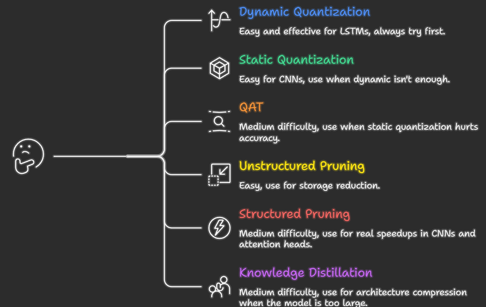
The Decision Framework: What to Use When

Stop guessing. Use this:

Is inference too slow?
    → Try dynamic INT8 quantization first (5 minutes of work)
    → If not enough: static INT8 with calibration
    → If GPU: consider FP16 (torch.cuda.amp) before INT8

Is the model too large to fit in memory or ship?
    → Quantization (INT8 shrinks 4×, INT4 shrinks 8×)
    → If still too large: distillation (train a smaller architecture)

Is accuracy dropping too much from quantization?
    → Switch to QAT (Quantization-Aware Training)
    → Use larger calibration dataset (>1000 samples)

Are you working with a CNN?
    → Structured channel pruning + static INT8

Are you working with an LLM (>1B params)?
    → INT4 via bitsandbytes (GPTQ for best accuracy)
    → Distillation if you can afford to train

Do you need maximum compression?
    → Full pipeline: distill → structured prune → QAT

What Most People Get Wrong

These are the mistakes that waste hours or quietly hurt your model:

1. Skipping batch norm fusion before quantizing PyTorch’s quantization expects batch norm layers to be fused with their adjacent conv layers. If you forget this, quantization is less effective and can even break inference.

# Always do this BEFORE quantization, not after
from torch.quantization import fuse_modules
# Fuse conv → batch norm → relu into a single efficient op
model = fuse_modules(model, [['conv1', 'bn1', 'relu'], ['conv2', 'bn2']])

2. Calibrating on training data instead of validation/production data If your model sees slightly different distributions in production (different camera, different demographics, different domain), calibration on training data sets wrong quantization ranges. Always calibrate on data that matches your production distribution.

3. Aggressive one-shot pruning Pruning 80% at once almost never recovers well. The network’s internal representations are interdependent — removing too many at once destroys structure that can’t be rebuilt. Always use iterative pruning with fine-tuning between steps.

4. Student architecture too small for distillation to work Distillation is not magic. If your student has 100× fewer parameters than the teacher and the task is complex, the student doesn’t have the capacity to represent what the teacher knows. Rule of thumb: start with a student that’s 4–10× smaller, not 100× smaller.

5. Expecting unstructured pruning to speed up inference This is the most common misconception. Sparsity on paper ≠ speedup in practice. Use structured pruning or accept that unstructured pruning is for storage savings only.

The Deeper Insight: Architecture Beats Optimization

Here is something the optimization literature doesn’t say loudly enough:

A well-designed small model almost always beats an aggressively optimized large model.

MobileNet (designed for efficiency) outperforms a pruned VGG on mobile inference. DistilBERT (designed via distillation) is more useful than quantized BERT-large in most applications.

Optimization techniques are powerful, but they’re not a replacement for thinking carefully about what architecture is right for your constraints from the beginning.

If you’re starting a new project and know you need to deploy on edge hardware, design for it from day one. If you’re stuck with an existing large model, now you know the toolkit to compress it.

Summary

Going deeper on quantization

This article covered the full optimization toolkit. If quantization was the technique that clicked most for you, there’s a lot more to explore, GPTQ (the algorithm behind most 4-bit LLMs), quantizing transformers from scratch, benchmarking INT4 vs INT8 vs FP16 on real hardware, and AWQ for activation-aware quantization. Those topics deserve their own dedicated walkthrough, so look out for that article next.

If this was useful, give it some claps — it helps other engineers find it.

Questions and feedback welcome in the comments.

How to shrink your ML model 9× and make it 6× faster was originally published in Level Up Coding on Medium, where people are continuing the conversation by highlighting and responding to this story.