Generating Random Numbers in Go

GoGo Tutorial

From simple tricks to advanced techniques that use inverse cumulative distribution functions

Table of Contents

• Summary
• Motivation
• Acronyms
• Using the Examples
• Random Number Sources
• Sample a Non-Negative Integer
• Sample a Float
• Sample from a Normal Distribution
• Sample from a Log-Normal Distribution
• Sample from an Exponential distribution
• Sample Elements from a Set using a Non-Uniform Probability Distribution
◦ Sampling Algorithm
• Sample a Subslice from a Larger Slice
• Shuffling the Elements of a Slice
• Sample from Arbitrary Distributions
• Sample from a Triangular Distribution
◦ Truncated Distribution
• Sample Points on Earth Using a Cosine Distribution
• The CLI Test Tool
• References

Summary

This article explains how you can sample random numbers and select random elements from a set using the Go language.

It begins by presenting simple sampling examples that use the Go standard library math/rand/v2 functions with almost no extra code. These examples cover sampling from the following distributions: uniform (discrete and continuous), normal, log-normal, and exponential.

The article then moves to examples that use more advanced techniques. These cover how you can randomly pick an enum from an enum set, i.e., select from a set with a discrete probability distribution; and how to build a subset from randomly selected elements of a larger set.

The final examples show you how to use an inverse cumulative distribution function (inverse CDF) to sample numbers from continuous distributions. This technique is the most advanced and the most powerful. The technique can be quite efficient when sampling from truncated distributions, where you only want to sample over a subset of the distribution domain. This is the most technical section of the article, but probably the most interesting.

We will sample numbers from a bounded triangular distribution using the triangular distribution’s inverse CDF. We will also explain how you can sample points with equal density on a sphere (e.g., Earth). For the points sampling, we will be using the inverse CDF of a cosine-based distribution function.

If you are already familiar with the functions of the math/rand/v2 package, you may still find the more advanced sections interesting, in particular the sections that discuss the inverse CDF.

All the code presented in this article is also available in a git repository at
https://gitlab.com/adrolet/randomgen_tutorial [1].

This repository provides a CLI application that you can run to experiment with each of the techniques presented below.

Note: The examples and libraries discussed here are suitable for general-purpose pseudo-random number generation, such as simulation. They should not be used for security-sensitive work where you have requirements for strong cryptography.

For cryptographically secure random number generators, you can start by exploring what the Go library crypto/rand [2] offers.

Motivation

In some applications, like games and simulations, you need to generate variations on inputs or on processing. This typically implies generating numbers that are bounded by some range and follow a probability distribution.

Acronyms

Here are a few acronyms that will be used in this article. The definitions below are adapted excerpts from Wikipedia.

PDF: Probability Density Function [3]

The Probability density function is a function whose value at any given sample (or point) in the sample space (the set of possible values taken by the random variable) can be interpreted as providing a relative likelihood that the value of the random variable would be equal to that sample. The value returned by the PDF is a probability density, abbreviated as PD in this article. A continuous PDF must be integrated over an interval to yield a probability.

PMF: Probability Mass Function [4]

A probability mass function is a function that gives the probability that a discrete random variable is exactly equal to some value. All the values returned by this function must be non-negative and sum up to 1.

A probability mass function differs from a continuous probability density function in that the latter is associated with continuous rather than discrete random variables.

CDF: Cumulative Distribution Function [5]

The cumulative distribution function is the probability that a real-valued random variable will take a value less than or equal to x. It is the integral of its probability density function from its lower bound of the sampling space (often 0 or -∞) to x. We can also define a CDF for discrete distributions, in which case the integral is replaced by the sum of the discrete probabilities.

Using the Examples

The following import should be included in all files that use one of the examples below.

import (
    ...
    "math/rand/v2"
    ...
)

The full documentation of the rand library is available at:
https://pkg.go.dev/math/rand/v2 [6]

Version 2 is used since it is an improvement over the original version. Version 2 provides new sources of random numbers: ChaCha8 and PCG. They bring significant enhancements to the unpredictability, security, and scalability of the generation process. In an attempt to stay focused, source discussions will be considered out of scope in this article, except for the basic source creation examples presented below.

Readers who want to know more should appreciate the following references.

• Evolving the Go Standard Library with math/rand/v2 [7]
• Secure Randomness in Go 1.22 [8]
• The ChaCha8 Pseudo-Random Number Generator is Now Standard [9]
  AI translation of a Chinese article.

Random Number Sources

The functions in math/rand/v2 can be called directly (package top-level functions) or from a source you created. The top-level functions use the Go runtime default source, a ChaCha8 source.

Here is how you could call a top-level function.

    rand.IntN(10000)

If you have a requirement to get the same sequence of random numbers for every application launch, you can seed a new source with a constant value at each launch. Once you have a source, you call the methods on the source, instead of prefixing the function’s name with the package name. Here is how you could create ChaCha8 and PCG sources and call IntN on them.

    // ChaCha8 example
    seed := [32]byte{1, 2, 3, 4, 5, 6, 7, 8, 9, 10, 11, 12, 13, 14, 15, 16, 17, 18, 19, 20, 21, 22, 23, 24, 25, 26, 27, 28, 29, 30, 31, 32}
    RandGen := rand.New(rand.NewChaCha8(seed))
    fmt.Printf("Fixed seed ChaCha8: IntN = %d\n", RandGen.IntN(10000))

    // PCG example
    seed1 := uint64(345673278749)
    seed2 := uint64(31415926535897932)
    RandGen := rand.New(rand.NewPCG(seed1, seed2))
    fmt.Printf("Fixed seed PCG: IntN = %d\n", RandGen.IntN(10000))

On the other hand, if you have a requirement to get a different sequence for every application launch, then you must create a source with a new seed each time. It is worth noting that from Go 1.22, the Go runtime provides something quite similar to the ChaCha8 example below. You therefore already get new seeds at each launch by default.

    import (
        cryptoRand "crypto/rand" // needed for ChaCha8 seed
        "fmt"
        "math/rand/v2"
        "time"                   // Needed for PCG seeds
    )

    // ChaCha8 example
    var seed [32]byte
    // func crnd.Read(b []byte) (n int, err error)
    // Read fills b with cryptographically secure random bytes.
    // It never returns an error, and always fills b entirely.
    _, _ = cryptoRand.Read(seed[:])
    RandGen := rand.New(rand.NewChaCha8(seed))
    fmt.Printf("New seed ChaCha8: IntN = %d\n", RandGen.IntN(10000))

    // PCG example
    seed1 := uint64(time.Now().UnixNano())
    seed2 := uint64(time.Now().UnixMicro()) * 31415926535897932 // just my own suggestion; be creative
    RandGen := rand.New(rand.NewPCG(seed1, seed2))
    fmt.Printf("New seed PCG: IntN = %d\n", RandGen.IntN(10000))

Sample a Non-Negative Integer

One of the simplest generation cases is the case where we want to sample random integers, and all numbers have an equal probability. A good example of this is simulating the rolling of a die to sample numbers from 1 to 6, or drawing balls for a Bingo game (assuming you map each ball to a number).

In this case, we are sampling from a Discrete Uniform distribution [10]. The graphic below depicts the probability mass function for this distribution when the sampling interval is bounded by a and b.

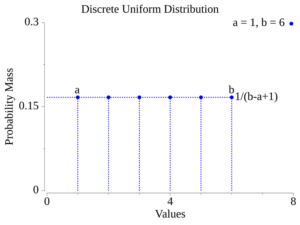
The Go library has functions to sample integers in the interval [0,∞], and functions to sample in a bounded interval [a,b].

To sample an int in the interval [0,∞] use the function Int.

    r := rand.Int() // r is of type int

CLI command: go run . Int
cmd_int.go

To get an output of a different integer type, including unsigned types, use the equivalent function that matches the type you want:

func Int32() int32
func Int64() int64
func Uint() uint
func Uint32() uint32
func Uint64() uint64

To select from a specific interval, you can use one of the XxxN(n) functions. All of these functions return a number in the half-open interval [0,n). By adding a number to the output, you can easily transform the interval into [a,b).

To select an int between a and b (b excluded), use:

    a := 2
    b := 50

    r := a + rand.IntN(b-a) // r is of type int

CLI command: go run . IntN -a 2 -b 50 # for an interval of [2,50)
cmd_intn.go

You can easily sample over an interval that covers negative numbers by specifying a negative a.

For a different integer type, use one of the equivalent functions:

func Int64N(n int64) int64
func UintN(n uint) uint
func Uint32N(n uint32) uint32
func Uint64N(n uint64) uint64

For a more generic approach, the library also offers the generic function N:

The input to N must satisfy the interface rand.intType, which is any type based on one of the following types: int, int8, int16, int32, int64, uint, uint8, uint16, uint32, uint64, uintptr.

    // As an example, here the arguments are uint64.
    a := uint64(34)
    b := uint64(245)

    // func N[Int intType](n Int) Int
    r := lowN + rand.N(b-a)

CLI Command: go run . N -a 5 -b 10
cmd_n.go

Sample a Float

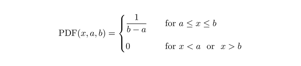
One of the most useful cases is the case where we want to sample floating-point numbers within some interval, and where all numbers have the same probability.

In this case, we are sampling from a Continuous Uniform distribution [11]. The graphic below depicts the probability density function for this distribution when the sampling interval is bounded by a and b.

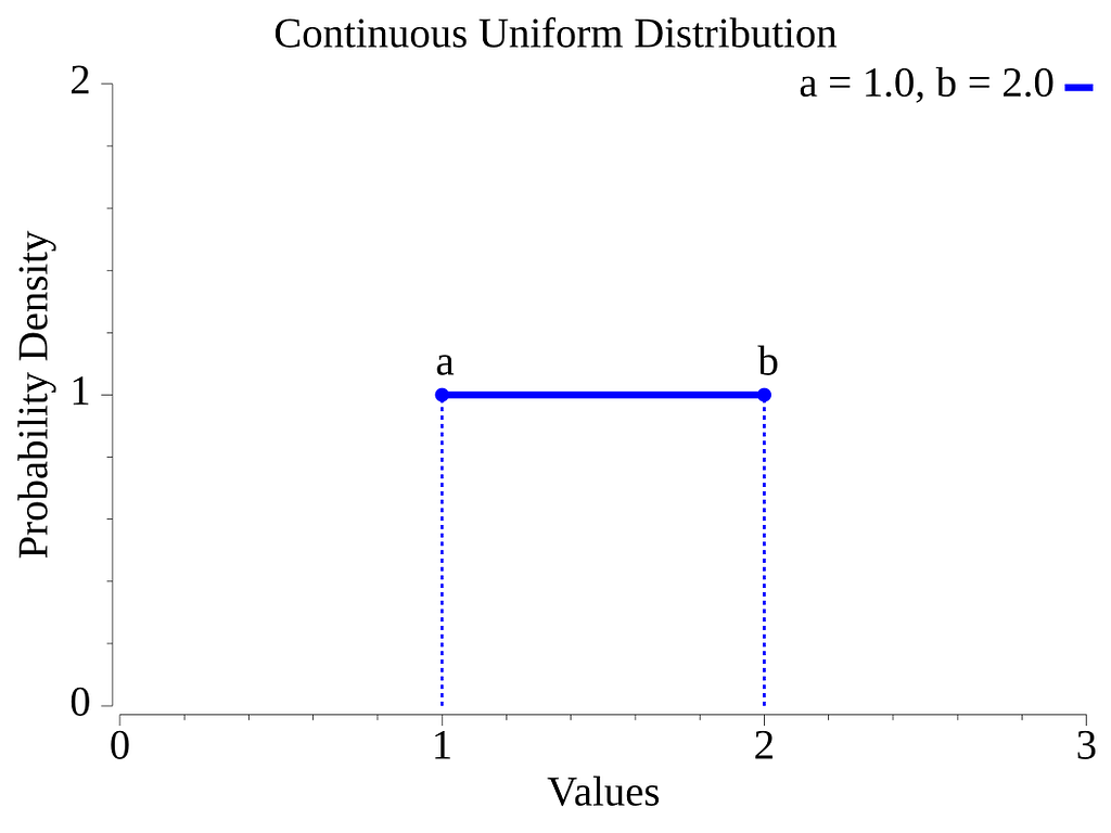
The Go library has two functions to sample floating point numbers in the half-open interval [0.0, 1.0), Float32 and Float64.

To adjust the interval to a custom [a, b) interval, simply multiply the function output by the interval width (b-a) and add the value of a.

    lowF64 := float64(-12.58)
    highF64 := float64(25.34)

    r := lowF64 + (highF64-lowF64)*rand.Float64() // r is of type float64

CLI command: go run . Float64 -a -12.58 -b 25.34
cmd_float64.go

Sample from a Normal Distribution

A quite popular probability distribution that shows up in many places is the Normal distribution [12]. The normal distribution has two parameters: a mean and a standard deviation (µ, σ). The graphic below illustrates the probability density function of the normal distribution for three sets of parameters.

The sample from a normal distribution, the Go standard library offers the function NormFloat64. It returns Float64 numbers that follow a normal distribution with a mean of zero and a standard deviation of one.

To adjust for a given parameter set, simply multiply the function output by the standard deviation, σ, and add the mean, µ, to the result.

    mean := float64(2)
    std := float64(0.5)

    r := mean + (rand.NormFloat64() * std) // r is of type float64

CLI command: go run . NormFloat -m 2 -s 0.5
cmd_norm.go

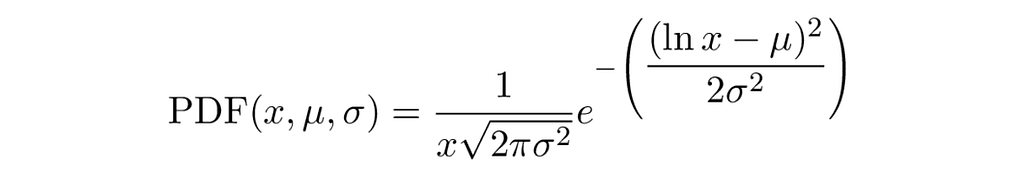
Sample from a Log-Normal Distribution

Another distribution that is often encountered when modeling size distributions (e.g., comment length, weights) or growth rates is the Log-normal distribution [13]. Numbers can be sampled from this distribution simply by using samples from a normal distribution and using them as the exponent to e.

The log-normal distribution is right-skewed [14], meaning it has a longer tail on the right side and its hump is on the left side. A right-skewed distribution has this relation between its mode, median, and mean: mode < median < mean. The domain of this distribution is limited to positive numbers. The log-normal distribution has two parameters. The parameters are the mean and standard deviation of the normal distribution used to create the samples.

The graphic below depicts the log-normal probability density function for three sets of parameters.

We can sample log-normal distributed numbers by using the functions NormFloat64 and Exp.

    normalMean := float64(0)
    normalStd := float64(1)
    nr := normalMean + (rand.NormFloat64() * normalStd)
    lnr := math.Exp(nr)

CLI command: go run . Lognorm -m 2 -s 1
cmd_lognorm.go

Sample from an Exponential distribution

The standard library also provides a function for the Exponential distribution [15], rand.ExpFloat64. The exponential distribution is a distribution where low values have the strongest probability of being sampled, while the probability decreases exponentially as the numbers get larger. This distribution can be used to model the time between two events in a Poisson point process [16]. This distribution has a single parameter, λ. Lambda acts as a scaling factor in the distribution. The mean of the distribution is: 1/λ.

The graphic below depicts the exponential probability density function for three values of λ.

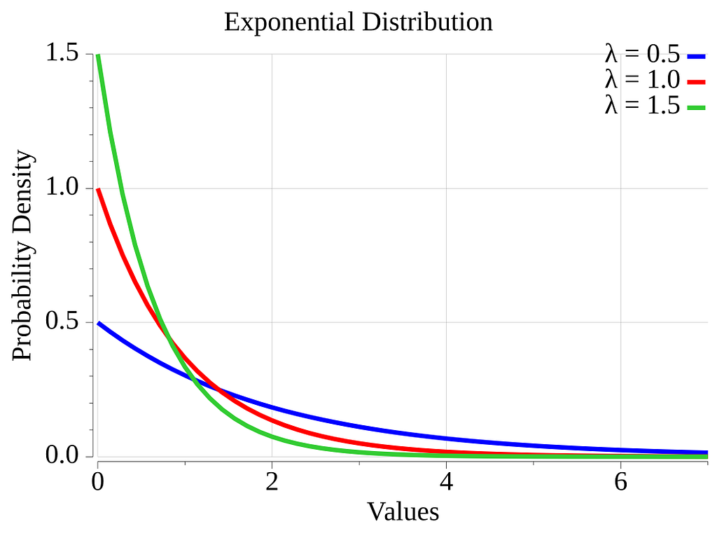
The Go function ExpFloat64() can be used as follows.

    lambda := float64(1.5)
    r := rand.ExpFloat64() / lambda

CLI command: go run . Exp -l 1.5
cmd_exp.go

Sample Elements from a Set using a Non-Uniform Probability Distribution

Now that we have covered the easy cases where the rand library is used almost as-is, let’s explore more complex usages.

In this section, we will explain how we could randomly sample elements from a set. The algorithm presented supports distributions that specify individual probabilities for each element.

Such sets could be enum sets that represent states or actions in a game or simulation. One example could be the moves an automaton can make on a grid. The move values could be: forward, backward, left, and right. Each move has its own probabilities: e.g., forward 40%, right and left 25% each, and back 10%. This involves sampling from a discrete non-uniform distribution.

So let’s see how we could model the enum sets and their distributions.

First, here is a simple distribution that only uses the basic type: int. It represents a distribution from which we can sample numbers from 1 to 5. We want a high probability of sampling 1, and lower probabilities of sampling larger numbers.

var SmallNumbersDistribution = map[int]int{
    1: 75,
    2: 10,
    3: 5,
    4: 5,
    5: 5,
}

The model is a Go map where the keys are the values in the enum set. Each enum value is associated with a weight stored as a map value.

The weights indicate the relative probability of sampling the enum value compared to the other values. The code does not require that the weights add up to 100. Later, we will see that the mass probability of a value is determined by dividing the value’s weight by the sum of all the weights in the distribution. As you can see, the distribution mass probabilities can be totally arbitrary. There is no need to have a nice equation that covers every enum value. More on this later.

Let’s look at two other examples. These distributions involve custom types

type CarState int

const (
    Parked CarState = iota + 1
    Stopped
    Rolling
)

var CarStateDistribution = map[CarState]int{
    Parked:  50,
    Stopped: 10,
    Rolling: 40,
}

type Move string

const (
    Forward  = Move("Forward")
    Backward = Move("Backward")
    Right    = Move("Right")
    Left     = Move("Left")
)

var MovesDistribution = map[Move]int{
    Forward:  40,
    Backward: 10,
    Right:    25,
    Left:     25,
}

The MovesDistribution demonstrates that an enum value type does not necessarily need to be a number type. A nominal/category [17], e.g., string-type, or any type acceptable as a map key (i.e., comparable) will also work.

Using a custom type adds type-safeness since it allows the compiler to validate that function arguments and variable values pertain to a given set. I.e., an arbitrary int cannot be confused with a CarState numerical value.

If you look at the CarState type definition in the randomgen_tutorial repo (cmd_enum.go), you will find the definition of a String method on the CarState type. It can be used to print a user-friendly name for each numerical value of the enum set.

Not depending on the weights to sum to 100 provides some freedom. It can make it easier to describe what you are modelling. Take the case of modelling a gumball machine. You could easily specify that it contains 254 blue balls, 189 red balls, and 302 yellow balls. There is no need for you to do the math. It can also help you to specify harder-to-approximate probabilities. E.g., weights of 33 and 66 (sum to 99) can be used to express 1/3 and 2/3. For higher precision, you could make the weights sum to something close to 1000 to get roughly 0.1% precision. If you need better, just update the code, replacing the map int values with float64 values. Update the rest of the code that expects an int. Should be trivial.

Sampling Algorithm

Now, here is the algorithm we will be using to sample the values.

To optimize performance, we will first sort the value-weight couples by descending weight in a slice. The benefits of doing this will become clear shortly.

Then we will determine the probability of sampling each value. As already mentioned, this is done by dividing the weight of a value by the sum of all weights.

Each value in the distribution can be seen as a segment of a line with a length equal to its probability. Placing these value segments one after the other builds up a longer segment with a length of 1. Let’s call this longer segment the all-values segment.

We can use the function rand.Float64 to generate a number in the interval [0,1). That number is then used to identify a position in the all-values segment, and therefore a point in one of the value segments. The longer the value segment, the higher the probability of the point being in that segment. So our algorithm is to select a random number between 0 and 1 and map it back to a value of the distribution.

On the all-values segment, the boundaries of the value segments are the cumulative probability (after the sorting) at each end of the value segments. For this reason, our generator will store the cumulative probabilities rather than the individual value probabilities.

That means that the probability we will store is the probability of a value, added to the probability of all the values previous to it in the sorted slice. The cumulative probability will be stored as a float64.

A function that maps a probability to a random value is called the inverse cumulative distribution function (inverse CDF). This important concept will be used more explicitly in the following sections on triangular and cosine distributions.

The following graphic should help you visualize the algorithm.

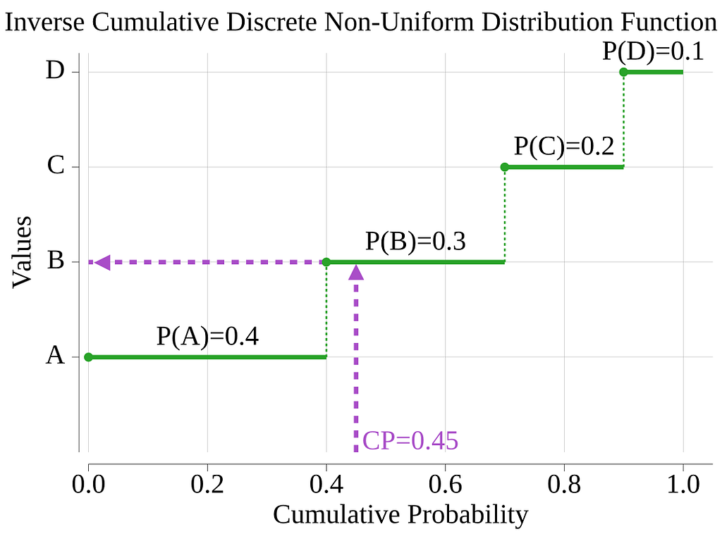
The sampling algorithm will generate a random number, then loop and test each value to see if the random number is less than or equal to the value’s cumulative probability. The first value that meets this criterion wins!

As the graphic illustrates, testing segments in descending order of probability maximizes the chance of an early match, decreasing the average number of loop iterations. For instance, with the above example, we will not test more than 2 values in 70% of the cases, while we will need to test the 5 values only in 10% of the cases. This optimization was an easy win!

This algorithm works very well for small sets. For sets with enough values to impact the performance of your application, you may want to replace the linear search loop with a better search algorithm. In comments I read on the web, someone indicated that a B-tree search could be used. I’m leaving it to the reader to improve as needed!

To implement this algorithm, we will use a struct type, a constructor, and a sampling method.

The struct that operates on the distribution information is called Sampler.

The use of generics allows the value type (T) to be types like: int, string, and much more.

type Sampler[T comparable] struct {
    values     []T
    cumulProbs []float64
}

To create an instance of it, one should use the constructor function, NewSampler.

func NewSampler[T comparable](distribution map[T]int) *Sampler[T] {

    type valNWeight struct {
        val    T
        weight int
    }

    var vwSlice = make([]valNWeight, 0, len(distribution))
    var totWeight int
    for v, w := range distribution {
        vwSlice = append(vwSlice, valNWeight{val: v, weight: w})
        totWeight += w
    }

    sort.Slice(vwSlice, func(i, j int) bool {
        // func(i, j int) bool{} is the `less` function used by the sort function for slices.
        // Here we want to sort from the largest weight to the smallest weight.
        return vwSlice[i].weight > vwSlice[j].weight
    })

    var values = make([]T, 0, len(distribution))
    var cumulProbs = make([]float64, 0, len(distribution))
    var lastCumul float64
    for _, vw := range vwSlice {
        values = append(values, vw.val)

        nextCumul := lastCumul + float64(vw.weight)/float64(totWeight)
        cumulProbs = append(cumulProbs, nextCumul)
        lastCumul = nextCumul
    }

    g := &Sampler[T]{
        values:     values,
        cumulProbs: cumulProbs,
    }

    return g
}

The valNWeight type is used to create a temporary slice where the distribution data can be sorted without losing the relationship between a value and its probability.

This function sorts the data by weight, converts the weights to cumulative probabilities, and then creates a new struct that contains a slice of values and a slice of cumulative probabilities.

Sampling of values from this sampler is done by calling the Val method on it.

func (s *Sampler[T]) Val() T {
    f := rand.Float64()
    for idx, l := range s.cumulProbs {
        if f <= l {
            return s.values[idx]
        }
    }
    return s.values[len(s.values)-1]
}

This is how you can create a distribution, create a Sampler, and use them.

    var SmallNumbersDistribution = map[int]int{
        1: 75,
        2: 10,
        3: 5,
        4: 5,
        5: 5,
    }

    sampler := NewSampler(SmallNumbersDistribution)
    
    fmt.Println(sampler.Val())

CLI command: go run . Enum -e smallNum
cmd_enum.go

Sample a Subslice from a Larger Slice

The rand library provides the function Perm(n int). This function returns a slice containing ints from 0 to n. The order of the numbers is randomized.

Calling rand.Perm(10)five times returns slices like:

[8 4 1 9 5 7 6 2 0 3]
[7 5 4 0 3 8 6 2 9 1]
[4 1 5 9 6 0 8 3 2 7]
[8 5 7 6 1 2 9 0 3 4]
[1 2 5 8 0 4 6 7 9 3]

One thing we can do with this is build subslices from a larger slice. Let’s suppose we have an original slice, M, with m elements, and we want to extract from it a subslice, N, with n elements. Of course, we must have 0 ≤ n ≤ m. We want the subslice to be made of a random selection of the elements in the original slice.

One possible algorithm for this is to create a slice, I, with the indices of all the elements of M. Next, we reorder the content of I randomly. Last, we pick the first n values of the randomized I, and use these indices to build the subslice N.

The first two steps are exactly what rand.Perm(n) does for us.

An implementation of this could look like this:

func Subslice[T any](M []T, n int) []T {
    // TODO consider returning an error for invalid n
    if n < 0 || n > len(M) {
        return M
    }

    // I, the first n index values in the randomize slice
    I := rand.Perm(len(M))[:n]

    N := make([]T, 0, n)
    for _, i := range I {
        N = append(N, M[i])
    }
    return N
}

func main() {
    M := []string{"A", "B", "C", "D", "E", "F", "G", "H"}
    n := 4

    N := Subslice(M, n)
    fmt.Println(N) // stdout: [C G D B]
}

In the above example, a slice made up of 8 string values is sampled to output a slice with 4 strings.

The algorithm is nicely wrapped in a generic function, Subslice. As you can see, the algorithm will work with slices of anything. In a shipping application, you probably want to enhance the handling of invalid arguments!

CLI command: go run . Subset -s 10
The Subset command outputs a subset of cards from a card deck. E.g., AS KS KH AH 9H JH 6H 5H 4D 3S.
cmd_subset.go

Shuffling the Elements of a Slice

In some cases, you may not want a subset of a slice, but instead just want to mix up a slice. For that particular case, you could consider the Shuffle function.

func Shuffle(n int, swap func(i, j int))

From the Go doc of Shuffle [18]:

Shuffle pseudo-randomizes the order of elements using the default Source. n is the number of elements. Shuffle panics if n < 0. Swap swaps the elements with indexes i and j.

The random library function Shuffle expects the number of elements to shuffle and a function that swaps two elements in a slice. You provide the swap function. Typically, this swap function will be a closure that has in its scope a reference to the slice to mix. Note that since it is your swap function that swaps elements based on indexes. Internally, you can handle any structure where the index makes sense to you, not just a slice.

The code below shows you how you could create your own Shuffle function wrapper.

    func Shuffle(myList []string) []string {
        rand.Shuffle(len(myList), func(i, j int) {
            myList[i], myList[j] = myList[j], myList[i]
        })
        return myList
    }

When applied to a slice, and given the way the above swap function is implemented, the backing store of the input slice myList is modified. Keep this in mind if the slice is referenced in many places, as the above swap function affects them all.

CLI command: go run . Shuffle -n 5 list-of-words
cmd_shuffle.go

Here is an example that shuffles a list of words 5 times.

% go run .  Shuffle -n 5 one two three four five six
[three five four two six one]
[two four six five one three]
[two three five four six one]
[five two one four six three]
[two four one three five six]

Sample from Arbitrary Distributions

In the next sections, we will see how we can use the inverse cumulative distribution function (inverse CDF) to sample numbers that follow any continuous distribution for which we can compute (or approximate) the inverse CDF. This is a very powerful technique.

The technique of using the inverse CDF is sometimes called inverse transform sampling. If you are interested in knowing more than what is presented in this article, you may start by reading this page on Wikipedia [19].

Digging the web with AI and Wikipedia, I found this definition of the inverse CDF:

The inverse cumulative distribution function, or quantile function F^-1(p), maps a probability p (between 0 and 1) to the corresponding value x of a random variable, such that P(X ≤ x) = p. It is used to find percentiles, critical values, and for generating random variables using inverse transform sampling.

Our first example that uses this technique will be about sampling from a triangular-shaped distribution. This simple distribution makes it easy to learn how to use the inverse CDF, since the mathematics for this distribution are easy to derive.

This example will be followed by a second one that uses a cosine-shaped distribution. This is not a typical probability distribution, but we will show how it can be used to sample well-distributed points on a sphere like the Earth.

Sample from a Triangular Distribution

Here, we will define a triangular probability distribution. To keep things simple, we will define its domain interval to be [0,1]. If needed, it can easily be moved and scaled to your requirements later. In our triangular distribution, the probability density (PD) starts with some value at one end of the interval, and changes linearly toward a different value at the other end of the interval. This linear change is what gives the distribution its triangular shape (for the purist, unless one end has a zero PD, this is a right trapezoid [20]).

The figure below displays the probability density function of two triangular distributions. The figure also presents their cumulative distribution function (CDF) curves, which we will derive shortly.

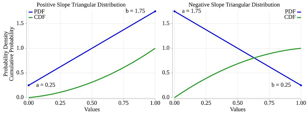
The parameters for this distribution are the a and b values. The parameter a indicates that we want numbers at the low end of the interval to be sampled with some arbitrary probability, and parameter b is used to indicate a different probability for the high end of the interval. As we are about to demonstrate, the absolute values of a and b are not important; only their relative values matter.

It is assumed that: 0 ≤ a, 0 ≤ b, and 0 < a+b.

In a software project I worked on, I had a slice of objects from which I wanted to randomly select some neighbors for each object. I wanted to bias my sampling so that I would pick more neighbors that were close to a given object, and pick fewer of the far neighbors. This distribution was perfect for my requirements.

We will now dig into some interesting math. If some of this stuff goes over your head, no problem, just skip to the inverse CDF equation, X(p_c, a, b), and look at its implementation in Go, cmd_triangle.go.

The PDF function, being a simple linear function, should look like this. Here we have temporarily introduced a scaling constant, k:

We will determine the formula for k by using the fact that the integration of a PDF over its domain must equal 1.

Therefore, the correctly scaled equation for our PDF is given by:s

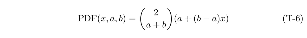
Note that choosing values for a and b that sum to 2 makes the scaling factor disappear.

Given this PDF function, let’s derive its cumulative sum, the CDF.

For this triangular distribution, the constant of integration, often denoted C, must be zero to ensure that the cumulative distribution function, CDF(b), sums to one. The next section, which introduces a cosine distribution, will provide an example where C evaluates to a non-zero value.

The CDF curves for the ramp-up and ramp-down examples are displayed in green in Fig. 8 above. We can see that they are segments of a parabola. The parabola can be convex or concave depending on the sign of the slope of the PDF.

We now know how to evaluate for a given value of the triangular distribution its cumulative probability. To implement the inverse transform sampling, we need a way to find the distribution value from a given cumulative probability. Basically, we need to derive the inverse CDF function.

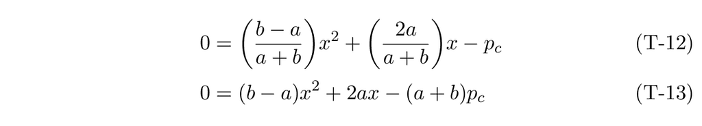
If we name the cumulative probability, p_c, and rewrite the equation so that it equals zero, we get.

Let’s rewrite this as a typical quadratic equation:

There is a well-known solution for the quadratic equation.

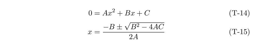
In our CDF equation, A, B, and C become:

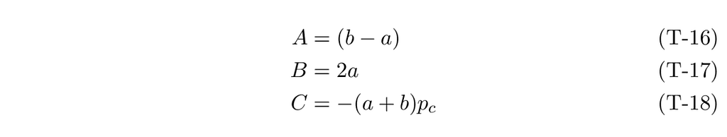
Applying this solution to our CDF function, we get:
We only keep the + option of the square root, since we know that x is in the interval [0,1] and therefore positive.

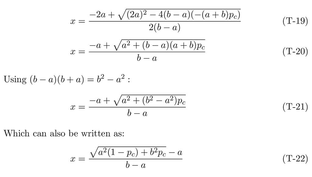
Our inverse CDF function, X(p_c, a, b), therefore, is:

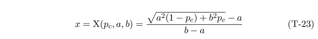
For pure triangular distributions, i.e., one with either a or b set to zero, we have these simplified CDF functions:

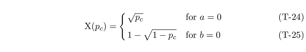
With this in mind, sampling simply becomes:

• Pick a random number in the interval [0,1]. Use it as a cumulative probability.
• Pass the cumulative probability to the inverse CDF function. What comes back is your sampled value from the distribution.

The next figure illustrates the algorithm.

We went through a lot of math, but in the end, we only care about the inverse CDF function, X(p_c, a, b). It is a simple function, and sampling from it can be done using code similar to the code below:

func TriangularInverseCdf(p, a, b float64) float64 {
    a2 := a * a
    b2 := b * b
    x := (math.Sqrt(a2*(1-p)+b2*p) - a) / (b - a)
    return x
}

func SampleTriangularDistribution(a, b float64) float64 {
    cp := rand.Float64()
    x := TriangularInverseCdf(cp, a, b)
    return x
}

CLI command: go run . Triangle -a 0.1 -b 1.0
cmd_triangle.go

All the above equations assume a distribution domain of [0,1]. Just like many examples in the previous sections, remember that you can always scale the interval and shift it to make it map to any interval your application requires.

This inverse sampling technique is general and, in theory, can be applied to any continuous distribution. In practice, however, some distributions have a complex PDF function that can be hard or impossible to integrate and invert analytically. That should not stop you. When an inverse function is not available, you can revert to numerical techniques to approximate the inverse CDF. For instance, you could use a set of functions to approximate, segment by segment, the real inverse CDF. You could also, using the CDF, compute couples made of the cumulative probability and distribution values, and store them in a table. To approximate the inverse CDF, you simply find the couples in the table that border what Float64 has returned and interpolate between the two couples. Numerical solutions are often not very hard to implement. Of course, this is typically slower than computing an inverse CDF, but you get an answer, and the complexity of the distribution function is no longer a show-stopper. Numerical solutions could fill an article by themselves. If a numerical solution is needed, it should not be very hard to find resources on the web that explain the various possible techniques.

Truncated Distribution

Sometimes you may want to sample a distribution over a subset of its domain. If the goal is only to cut the extremes of a distribution, like cutting the thin tails of a normal, then an easy technique is to sample normally, test the sampled value, and drop and re-sample if the value is outside the desired interval. If the drop rate is low enough (e.g., < 1%), then resampling remains efficient.

When resampling becomes too costly, you can use the inverse sampling technique to only sample the desired portion of the domain.

To do so, you need to know the cumulative probabilities, CPs, of the ends of the desired interval. In some cases, you may not know the CPs but have the end values of the subdomain; in this case, use the CDF function to compute the CPs or compute some estimations of them numerically.

Once you have the end CPs, massage the output of rand.Float64 to fit the sub-domain. Then feed these massaged CPs into the inverse CDF.

This could look like:

    lowCp := float64(0.2)
    highCp := float64(0.6)
    cp := lowCp + (highCp-lowCp)*rand.Float64()
    value := myInverseCdf(cp)

The next section shows how to sample points on Earth and uses truncation.

Sample Points on Earth Using a Cosine Distribution

In this section, we will use what we have learned so far to solve a problem that goes beyond simple random number generation.

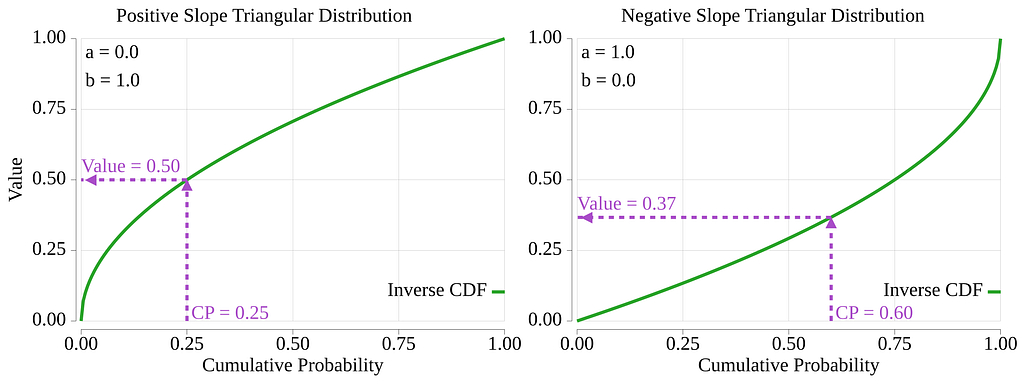
Let’s say that we are writing an application that involves geography, and that we want to randomly select points on Earth. The proposed solution will involve inverse sampling. To make it more fun, we will also use truncation techniques to limit the sampled points to a bounded area delimited by a pair of meridians and a pair of parallels, a spheroidal quadrangle [21], aka bounding box.

We also want the sampled points to be equally dispersed over the bonded area. This will bring a cosine-based distribution into the equation.

Our problem involves sampling in two dimensions, not just one as we have done so far, and the surface is not Euclidean; it is a sphere.

The solution will therefore include sampling of longitudes over the domain of [-180, +180] degrees. It will also include a sampling of latitudes over the domain [-90, +90] degrees. As we are about to see, our “equally dispersed” constraint will make this, let’s say, more interesting.

The figure below should aid in visualizing the geometry of the problem.

To sample a point, we will first sample a longitude. Since all longitudes are equally acceptable, we can use a uniform continuous distribution to sample the longitude. We simply need to resize the output domain of rand.Float64, from [0, 1], to [-π, +π] radians.

The implementation of the longitude sampling function is presented further down with the latitude functions.

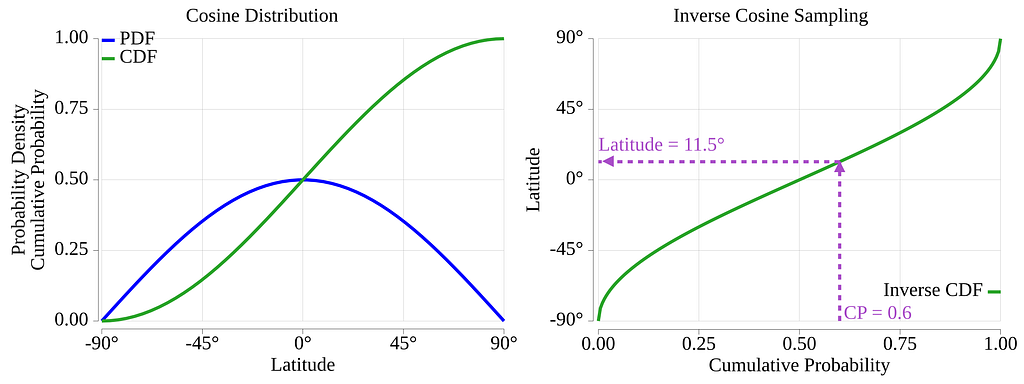
The sampling domain for the latitudes is [-π/2, +π/2] radians. If we were to sample it using a uniform distribution, we would get, on average, the same number of points for any equal-width latitude band. Such bands on a sphere are called zones [21]. Here, we need to recognize that the circumference of the circle created by the intersection of the parallel plane with the Earth’s sphere is a function of the latitude. It is obvious that the parallel at the equator has the largest circumference, and that the parallel at latitude +85º has a much smaller one. Now, if we had a similar number of points for each equal-width zone, this would create a high concentration of sampled points near the poles, and a much lighter concentration near the equator. Given our “equally dispersed” requirement, we need to fix this.

To fix this, we will use a distribution that is proportional to the circumference of the parallel. Therefore, sampling more often the equatorial region and less often the polar regions.

In the next equations, R is the radius of the Earth, and r is the radius of a parallel circle for a given latitude, i.e., the distance, perpendicular to the rotation axis, between the parallel on the Earth’s sphere and its axis.

Now that we have an idea of the PDF equation, we will follow the same steps as for the triangle distribution in the above section: scale the PDF, derive its CDF, and derive its inverse CDF.

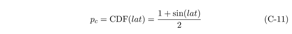
Our PDF, therefore, is:

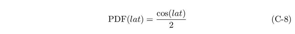
From which we derive the cumulative probability, p_c, and its function, CDF(lat):

Where C is the constant of integration. In the triangular distribution, it was zero. We know that a CDF must be equal to zero at the beginning of its domain and one at the end. For the cosine case, with a C of zero, we would have: CDF(-π/2) = -1/2 and CDF(π/2) = 1/2. From this, we can see that we must set the value of C to 1/2 to get the correct range for the CDF function.

Our final CDF equation is therefore:

Isolating lat, we get our inverse CDF, Lat(p_c).

Just like for the triangle distribution, once the math is done, implementing inverse sampling is pretty simple. In a first step, let’s look at an implementation that does not consider bounding the sampling within a latitude interval.

    func BoundlessSampleLatitude() float64 {
        cp := rand.Float64()       // sample a cumulative probability
        rad := math.Asin(2*cp - 1) // apply the inverse CDF
        return rad * 180 / math.Pi // convert to degrees
    }

Now that we have the basics, let’s add code that limits the sampling to a latitude interval. Most likely, you will want to specify the interval in terms of latitudes, not cumulative probabilities. The inverse CDF function, however, consumes cumulative probabilities, so we must first convert our latitude boundaries in degrees to cumulative probability boundaries. We can do this with the CDF function. Then we can generate a random sample within this probability interval and convert the probability back to a latitude in degrees. The code could look like this:

    // CosCdf returns the cumulative probability of lat for a cosine distribution.
    func CosCdf(lat float64) float64 {
        radLat := lat * math.Pi / 180
        cp := (1 + math.Sin(radLat)) / 2
        return cp
    }

    // SampleLatitude returns a random latitude in the interval [minLat, maxLat].
    func SampleLatitude(minLat, maxLat float64) float64 {
        minCP := CosCdf(minLat)
        maxCp := CosCdf(maxLat)

        cp := minCP + ((maxCp - minCP) * rand.Float64()) // sample a cumulative probability
        rad := math.Asin(2*cp - 1)                       // apply inverse CDF

        return rad * 180 / math.Pi // convert radians to degrees
    }

Putting it all together, and adding the function that samples the longitude, we get:

    // SampleLongitude returns a random longitude in the interval [minLong, maxLong].
    func SampleLongitude(minLong, maxLong float64) float64 {
        long := minLong + ((maxLong - minLong) * rand.Float64())
        return long
    }

    // SampleEarth randomly selects a point on Earth within the quadrangle formed by the arguments.
    func SampleEarth(minLat, maxLat, minLong, maxLong float64) (float64, float64) {
        lat := SampleLatitude(minLat, maxLat)
        long := SampleLongitude(minLong, maxLong)
        return lat, long
    }

CLI command: go run . Earth -n 10 — min-long 10 — max-long -150 — min-lat 45 — max-lat 90
cmd_earth.go

The Earth command produces a CVS output that can easily be imported by graphic packages. E.g.

% go run . Earth -n 10 --min-long 10 --max-long -150 --min-lat 45 --max-lat 90
lat,long
   49.5181,    4.9054
   60.3442,  -11.8683
   57.1618, -117.8188
   75.3065,  -62.3137
   56.3833,   -4.4709
   45.3452,  -55.7613
   61.8719,  -74.3986
   46.4397,   -8.0517
   73.1115, -135.4342
   53.1336,  -45.1114

Be aware that when sampling an area that crosses the ±180° meridian, the above math will get confused. Say that you want to sample an area that covers the Pacific Ocean, e.g., from the coast of China, roughly the -120° meridian, to Los Angeles, roughly the +120° meridian. If we remember that the whole longitude thing cycles every 360°, then one way to solve this is to subtract 360° from Los Angeles. This way, you can specify -min-long -240 and --max-long -120. A quick test indicates that this trick seems to work after you bring back the sampled longitude into the [-180, +180] interval. I did not spend a lot of time validating weird specifications. If similar code is used in production, make sure to validate all ranges and cover cases that cross the ±180° meridian.

The CLI Test Tool

To help you experiment with the techniques presented in this article, I created a repo that contains all the above examples wrapped in a small application. The application presents a command line interface (CLI), where each example can be executed by calling its sub-command name and providing its parameters.

The MIT-licensed repo can be cloned from
https://gitlab.com/adrolet/randomgen_tutorial

You can get the list of sub-commands by running the app with the -h, ‑‑help flag. All commands support the -n flag. It is used to specify the number of samples you want to output. If not specified, a single sample is returned.

% go run . --help
Usage:
  randomgen_tutorial [command]

Available Commands:
  Earth       Returns a pseudo-random point on Earth (lat, long)
  Enum        Returns a value from an enum distribution
  Exp         Returns an exponentially distributed float64 in the half-open interval (0, +math.MaxFloat64]
  Float64     Returns a pseudo-random float64 in the half-open interval [a, b)
  Int         Returns a non-negative pseudo-random int
  IntN        Returns a pseudo-random int in the half-open interval [a,b)
  Lognorm     Returns a log-normal distributed float64
  N           Returns a pseudo-random int in the half-open interval [a,b)
  Norm        Returns a normal distributed float64
  Shuffle     Returns the list of line arguments in a random order
  Subset      Returns a subset of a card deck
  Triangle    Returns a pseudo-random float64 from a triangular distribution with parameters: a, and b
  completion  Generate the autocompletion script for the specified shell
  help        Help about any command

Flags:
  -h, --help      help for randomgen_tutorial
  -v, --version   version for randomgen_tutorial

Use "randomgen_tutorial [command] --help" for more information about a command

Here are two examples of commands you can run.

Sampling from a normal distribution:

% go run . Norm -h
Returns a normal distributed float64 in the range [-math.MaxFloat64, +math.MaxFloat64] with mean of -m and stddev of -s

Usage:
  randomgen_tutorial Norm [flags]

Flags:
  -h, --help             help for Norm
  -m, --mean float       The mean of the distribution (default 0)
  -n, --num-sample int   The number of samples to output (default 1)
  -s, --std float        The standard deviation of the distribution (default 1)

% go run . Norm -n 5 -m 2.5 -s 0.5
3.0467274614
2.4353416499
1.8573580946
2.3208547901
3.3999356776

Sampling from our triangular distribution:

% go run . Triangle -h
Returns a pseudo-random float64 from a triangular distribution

Usage:
  randomgen_tutorial Triangle [flags]

Flags:
  -a, --aParam float     The probability density at 0.0 (default 0)
  -b, --bParam float     The probability density at 1.0 (default 1)
  -h, --help             help for Triangle
  -n, --num-sample int   The number of samples to output (default 1)


% go run . Triangle -a .1 -b 1.5 -n 5
0.5831363456
0.5666553034
0.4916918980
0.3179371236
0.7990433852

This repo is for you to experiment. Feel free to fork it and make any changes needed to fit your requirements.

References

[1] randomgen_tutorial git repository. It hosts the demo CLI application
https://gitlab.com/adrolet/randomgen_tutorial

[2] The crypto/rand Go standard library
https://cs.opensource.google/go/go/+/refs/tags/go1.25.6:src/crypto/rand/

[3] Probability Density Function
https://en.wikipedia.org/wiki/Probability_density_function

[4] Probability Mass Function
https://en.wikipedia.org/wiki/Probability_mass_function

[5] Cumulative Distribution Function
https://en.wikipedia.org/wiki/Cumulative_distribution_function

[6] The math/rand Go standard library
https://pkg.go.dev/math/rand/v2

[7] Evolving the Go Standard Library with math/rand/v2
https://go.dev/blog/randv2

[8] Secure Randomness in Go 1.22
https://go.dev/blog/chacha8rand

[9] The ChaCha8 Pseudo-Random Number Generator is Now Standard.
AI translation of a Chinese article
https://zenn.dev/spiegel/articles/20240309-golang-math-rand-v2?locale=en

[10] Discrete uniform distribution
https://en.wikipedia.org/wiki/Discrete_uniform_distribution

[11] Continuous uniform distribution
https://en.wikipedia.org/wiki/Continuous_uniform_distribution

[12] Normal distribution
https://en.wikipedia.org/wiki/Normal_distribution

[13] Log-normal distribution
https://en.wikipedia.org/wiki/Log-normal_distribution

[14] Skewness
https://en.wikipedia.org/wiki/Skewness

[15] Exponential distribution
https://en.wikipedia.org/wiki/Exponential_distribution

[16] Poisson point process
https://en.wikipedia.org/wiki/Poisson_point_process

[17] Types of data
https://www.brookes.ac.uk/students/academic-development/maths-and-stats/statistics/types-of-data

[18] Go doc for the function Shuffle
https://pkg.go.dev/math/rand/v2#Shuffle

[19] Inverse transform sampling
https://en.wikipedia.org/wiki/Inverse_transform_sampling

[20] Right Trapezoid
https://lexique.netmath.ca/en/right-trapezoid

[21] quadrangle, zone, and lune (See bottom of page)
https://www.mathworks.com/help/map/ref/areaquad.html

Generating Random Numbers in Go was originally published in Level Up Coding on Medium, where people are continuing the conversation by highlighting and responding to this story.