
There’s a peculiar irony in modern NLP: as models grow more powerful, the engineers who truly understand the foundations grow rarer. Everyone wants to fine-tune a BERT or deploy a GPT wrapper. Far fewer can answer the question that actually separates strong ML engineers from the rest:
Why do certain features work, and when do you use which?
This article isn’t a glossary. It’s a mental model — a way of thinking about how information in text gets compressed, transformed, and ultimately handed to a machine that has no idea what a word even is.
Let’s build that understanding from the ground up.
The Fundamental Problem: Bridging Two Worlds
A model is, at its core, a mathematical function. It takes numbers in, produces numbers out. Text is not numbers. So the first question in any NLP system isn’t “which model?” — it’s “how do I make this text legible to a function?”
That’s what feature engineering is. It’s translation.
And every translation involves a choice about what to preserve and what to discard. Word order? Meaning? Frequency? Context? Each feature type answers this question differently, and those tradeoffs define when each one is useful.
Let’s walk through them in the order you’d reach for them — from blunt instruments to precision tools.
1. Lexical Features: The Surface of Language
Before you even think about words as units of meaning, you can learn a lot from text’s physical shape.
Lexical features are surface-level statistics: word count, character count, average word length, ratio of uppercase letters, punctuation density, stopword proportion.
These sound almost embarrassingly simple. But consider what they capture:
- A phishing email often has unusual capitalization patterns and excessive punctuation
- A bot-generated review tends to have unnaturally uniform sentence length
- Formal documents have longer average word length than casual conversation
For classification tasks where style matters as much as substance — spam detection, bot identification, authorship attribution — lexical features punch well above their weight.
The deeper insight: These features are model-agnostic and near-zero cost to compute. In any production system, they’re always worth including as a baseline signal. The question isn’t whether to use them, but whether they’re sufficient alone.
They’re not. But they’re a foundation.
2. Bag of Words: Discarding Order, Keeping Presence
Bag of Words (BoW) makes a deliberate sacrifice: it throws away word order entirely, keeping only the frequency of each word across a fixed vocabulary.
Your sentence becomes a vector. The vocabulary defines the dimensions. Each dimension tells you how many times that word appears.
Vocabulary: ["machine", "learning", "is", "fun", "hard"]
Sentence:   "machine learning is fun"
Vector:     [1, 1, 1, 1, 0]
Why would you give up word order? Because for many tasks, order doesn’t matter much. A document about “machine learning” contains those words at high frequency regardless of how they’re arranged. Sentiment, topic, and category classification are often robust to order removal.
The real limitation of BoW isn’t the missing order — it’s the sparsity.
If your vocabulary has 50,000 words (modest by real-world standards), every document becomes a 50,000-dimensional vector where the vast majority of values are zero. This is computationally expensive to store and propagate, and statistically thin — most of that space is empty signal.
BoW also treats “not good” and “good” as nearly identical. The negation is lost. The sarcasm is lost. The semantic relationship between words is completely absent.
Despite this, BoW with Logistic Regression or Naive Bayes remains a competitive baseline. Its simplicity is a feature, not a bug, when you need interpretability or are operating under compute constraints.
3. TF-IDF: Teaching the Model About Rarity
The fundamental flaw BoW exposes is that not all words carry equal information. “The” appears in almost every document and tells you almost nothing. “Blockchain” appearing in a document tells you quite a lot.
TF-IDF formalizes this intuition with two components:
Term Frequency (TF): How often does this word appear in this document?
Inverse Document Frequency (IDF): How rare is this word across all documents?
The product gives you a weight that is high when a word appears frequently in a specific document but rarely across the corpus. This surfaces the words that are distinctively important to that document — not just common in general language.
TF("transformer", doc) = 0.05   # appears 5% of words
IDF("transformer", corpus) = 4.2  # rare across all docs
TF-IDF = 0.05 × 4.2 = 0.21
vs.
TF("the", doc) = 0.08
IDF("the", corpus) = 0.1  # appears in virtually every doc
TF-IDF = 0.08 × 0.1 = 0.008
The word “the” is penalized to near-zero. “Transformer” is rewarded.
Where TF-IDF still shines: document classification, keyword extraction, and any task where the subject of a document matters more than the meaning of individual sentences. It’s the backbone of older information retrieval systems and still a go-to for interpretable feature pipelines.
Its blind spot: TF-IDF still doesn’t understand that “car” and “automobile” mean the same thing. Two synonyms are two entirely separate dimensions in the vector space, with no relationship to each other. That’s where embeddings come in — but we’re not there yet.
Example:
Our tiny corpus (3 documents):
- Doc 1: “dog runs fast”
- Doc 2: “cat runs fast”
- Doc 3: “dog eats food”
We’ll calculate TF-IDF for the word “dog” in Doc 1.
Step 1: Calculate TF (Term Frequency)
How many times does “dog” appear in Doc 1, divided by total words in Doc 1.
TF = 1/3 = 0.33
Step 2: Calculate IDF (Inverse Document Frequency)
How many documents contain the word “dog”? Doc 1 and Doc 3. So 2 out of 3 documents.
IDF = log(Total Documents / Documents containing "dog")
IDF = log(3/2)
IDF = log(1.5)
IDF = 0.17
Step 3: Multiply them
TF-IDF = TF x IDF
TF-IDF = 0.33 x 0.17
TF-IDF = 0.056
Now let’s do the same for the word “runs” in Doc 1 to see the difference.
“runs” appears in Doc 1 and Doc 2, so again 2 out of 3 documents. TF is also 1/3. Looks the same so far.
But what if we tried the word “fast”? It also appears in Doc 1 and Doc 2. Same score.
Now try “eats”. It only appears in Doc 3, so it would get a higher IDF score there because it’s rarer.
The key point to see here:
If a word appeared in all 3 documents, the IDF would be log(3/3) = log(1) = 0. Multiply anything by zero and you get zero. That word gets completely suppressed, which is exactly what happens to stop words like “the” or “is” in a large corpus.
The rarer the word across documents, the higher its IDF, and the more it stands out as something meaningful and distinctive about that specific document.
Stop Words
We need to talk about something called Stop words at this point to explain when it is needed and when it is not.
For Bag of Words, stop words are removed before building the vocabulary.
Words like “the”, “is”, “a”, “and” appear in literally every sentence. If you keep them, they take up dimensions in your vector but carry zero useful information. They just add noise. So you strip them out first, and your vocabulary becomes cleaner and smaller.
Example:
“I love machine learning” becomes “love machine learning” after removing stop words. The word “I” tells the model nothing useful about what this sentence is about.
For TF-IDF, stop words are less of a problem because the math handles them automatically.
Since “the” appears in almost every document, its IDF score drops close to zero. Multiply that by any term frequency and the final weight is still basically zero. TF-IDF naturally suppresses stop words without you having to remove them manually.
But here’s the thing: most people still remove stop words before applying TF-IDF anyway. Why? Because keeping them wastes memory and compute time. Even if their weight is near zero, they still occupy space in a potentially 50,000 dimension vector. Removing them upfront just makes the whole pipeline leaner.
The simple takeaway:
Stop word removal is essential for Bag of Words because there’s nothing else to handle them. For TF-IDF it’s technically optional, but still good practice for efficiency. Think of it as cleaning your data before cooking, even if the heat would eventually kill the bacteria anyway. Better to not have it there in the first place.
4. N-grams: Local Context at Low Cost
Both BoW and TF-IDF treat every word as an island. N-grams introduce a minimal but meaningful form of context: consecutive word sequences.
- Unigram: "machine", "learning"
- Bigram: "machine learning", "is fun"
- Trigram: "machine learning is", "learning is fun"
The value becomes obvious when you consider what single words lose. “Not good” has the opposite sentiment of “good,” but a unigram model treats them as nearly equivalent. A bigram model captures “not good” as its own unit.
In practice, bigrams are often the sweet spot. Trigrams add marginal value and multiply your vocabulary size dramatically.
One important subtlety about vocabulary explosion:
If you have a vocabulary of V words, bigrams potentially add V² new terms. Most of those bigrams never appear in real text, but you still need to account for them. This is why N-gram models are typically combined with aggressive pruning — only keeping N-grams that appear above some minimum frequency threshold.
N-grams work especially well for tasks with important local phrasing: named entity recognition, chunking, and any domain where specific multi-word terms matter (medical NLP, legal documents, technical documentation).
5. Term Coverage and Matching Features: The Retrieval Perspective
In search and question-answering systems, you’re often asking a different question than “what is this document about?” You’re asking: how well does this document answer this query?
Term coverage features address this directly:
Query:    "best machine learning course for beginners"
Document: "a comprehensive machine learning tutorial for newcomers"

Query term coverage = (matched terms) / (total query terms)
Words like “machine learning” overlap. “Best” matches “comprehensive” only at the semantic level — term coverage at the lexical level won’t catch that. This is a real limitation.
But lexical overlap is cheap, fast, and surprisingly effective. In multi-stage retrieval systems (which we’ll discuss in a moment), term coverage serves as a powerful first-stage signal before you deploy expensive semantic models.
Other features in this family: exact match count, longest common subsequence, character-level overlap (catches morphological variants like “learn” and “learning”), Jaccard similarity.
When these matter most: ranking systems where you have a query-document pair and need a quick, interpretable relevance signal. Don’t underestimate them.
Example
You type a search query and the system checks how well a document covers your query terms.
Query: “best python course for beginners”
Total query words (ignoring stop words): “best”, “python”, “course”, “beginners” = 4 terms
Document 1: “This is the best python course you will ever take”
Matched terms: “best”, “python”, “course” = 3 out of 4
Term Coverage = 3/4 = 0.75 (75%)
Document 2: “A beginner friendly python tutorial”
Matched terms: “python”, “beginners” (tutorial matches course loosely but not exactly) = 2 out of 4
Term Coverage = 2/4 = 0.50 (50%)
Document 3: “best python course designed specifically for beginners”
Matched terms: “best”, “python”, “course”, “beginners” = 4 out of 4
Term Coverage = 4/4 = 1.0 (100%)
So the ranking would be:
Document 3 ranks first, Document 1 second, Document 2 third.
The important limitation to notice here:
Document 2 used the word “tutorial” instead of “course” and “beginner friendly” instead of “beginners.” A human reading it would say it’s clearly relevant. But term coverage doesn’t understand synonyms, it only looks for exact word matches.
That’s exactly why search systems pair term coverage with embedding similarity. Term coverage handles exact matches fast and cheap. Embeddings catch the semantic meaning that exact matching misses.
6. BM25: The Algorithm That Powers Most Search Engines
If you’ve used Elasticsearch, Apache Solr, or most major document retrieval systems, you’ve used BM25. It powers more production search than almost any other single algorithm, including most neural approaches.
BM25 extends TF-IDF with two critical improvements:
1. Term frequency saturation: In raw TF-IDF, if a word appears 100 times instead of 10, it gets 10× the weight. But intuitively, the 100th mention of a word adds less information than the 10th. BM25 introduces a saturation parameter (k₁) that dampens this relationship — early occurrences matter a lot, additional occurrences matter less.
2. Document length normalization: A long document will contain more of any given term simply because it has more words. BM25 normalizes by document length, preventing long documents from getting unfair advantage purely from their size.
The formula is:
BM25(D, Q) = Σ IDF(qᵢ) × [f(qᵢ, D) × (k₁ + 1)] / [f(qᵢ, D) + k₁ × (1 - b + b × |D|/avgdl)]
Where f(qᵢ, D) is term frequency, |D| is document length, avgdl is average document length, and k₁ and b are tunable parameters.
Why BM25 still dominates in 2026: It requires no training data, no GPU, and no model serving infrastructure. It runs in milliseconds on billions of documents. And it’s remarkably competitive against much heavier methods on sparse retrieval benchmarks.
The standard pattern in modern systems: use BM25 as first-stage retrieval to get a candidate set (top 100–1000 documents), then use neural re-rankers to refine that set. BM25 is the efficient filter; the neural model is the precision instrument.
7. Linguistic and Statistical Features: Structure as Signal
Natural language has deep structure that goes beyond word frequencies. Linguistic features let you exploit that structure.
Part of Speech Tags:
Part-of-Speech (POS) tags encode the grammatical role of each word. Knowing that a word is a verb versus a noun changes its interpretation entirely. In sentiment analysis, knowing that “disappointing” is an adjective modifying a noun helps you link it correctly. In information extraction, knowing the subject-verb-object structure helps you find relationships.
POS tagging just labels every word in a sentence with its grammatical role.
Sentence: “Apple launched a new phone yesterday”

Now how do you turn this into a feature?
The simplest way is to count how many of each POS tag exists in the sentence.
Noun count      = 2
Verb count      = 1
Adjective count = 1
Adverb count    = 1
Determiner      = 1
These counts become numbers you append to your feature vector alongside your TF-IDF or Bag of Words features.
feature vector = [tfidf values..., noun_count=2, verb_count=1, adj_count=1, adv_count=1]
Named Entity Recognition
Named Entity Recognition (NER) identifies and classifies proper nouns: people, organizations, locations, dates, products. A sentence containing “Apple” means something very different if “Apple” is tagged as an organization versus a fruit. NER gives you that disambiguation.
Example:
NER first identifies and labels specific entities in your text.
Sentence: “Elon Musk announced that Tesla will open a new factory in Berlin next year”

Now how do you actually feed this into a model?
There are a few simple ways.
Approach 1: Count based features
Just count how many of each entity type appears in the document.
PERSON count       = 1
ORGANIZATION count = 1
LOCATION count     = 1
DATE count         = 1
These counts get appended directly to your feature vector.
feature vector = [tfidf values..., person=1, org=1, location=1, date=1]
This is simple and works surprisingly well for document classification. A news article about politics will have high PERSON counts. A financial report will have high ORGANIZATION and DATE counts. A travel blog will have high LOCATION counts.
Approach 2: Replace entities with their labels
Instead of keeping the actual words, you replace them with their entity type before feeding into the model.
Original:
"Elon Musk announced Tesla will open a factory in Berlin"
After replacement:
"PERSON announced ORGANIZATION will open a factory in LOCATION"
Now when you run TF-IDF on this, the model learns patterns around entity types rather than specific names. This is powerful because the model learns that “PERSON announced ORGANIZATION” is a common pattern in business news, regardless of which specific person or company it is.
Approach 3: Binary flags
Sometimes you just want to know whether a certain entity type is present at all, not how many times.
has_person       = 1
has_organization = 1
has_location     = 1
has_money        = 0
has_date         = 1
This works well when the presence of an entity type matters more than its frequency.
A real world example putting it together:
Say you’re building a news article classifier to predict the category: Politics, Sports, Finance, or Travel.
Your feature vector for one article might look like this:
[
  tfidf values...,
  person_count    = 3,
  org_count       = 2,
  location_count  = 1,
  date_count      = 2,
  money_count     = 0,
  has_person      = 1,
  has_org         = 1,
  has_location    = 1
]
Over thousands of articles the model learns that high person count plus high org count usually means Politics or Business. High location count with low money count leans toward Travel. High money count with high org count points to Finance.
Dependency Parsing
Dependency parsing gives you the grammatical relationships between words — what modifies what, what’s the subject, what’s the object. This is expensive to compute but powerful for tasks that require understanding sentence structure, like question answering and relation extraction.
Example
Sentence: “The cat quickly ate the fish”
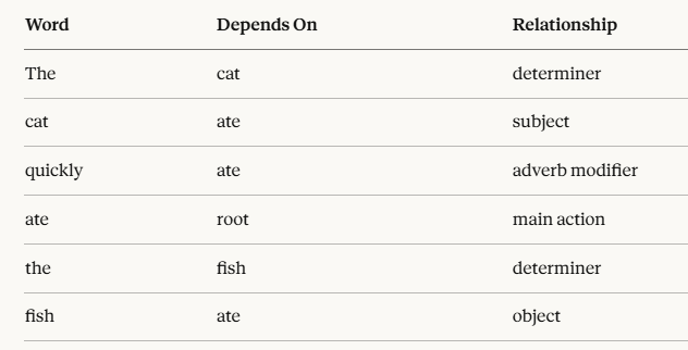
So the tree looks like this:
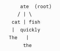
. cat is the one doing the action (subject)
. fish is what is being acted on (object)
. quickly describes how the action happened
Now how do you turn this into features?
Approach 1: Extract subject verb object triplets
Pull out the core relationship from every sentence as a triplet.
Subject = cat
Verb    = ate
Object  = fish
Feature: (cat, ate, fish)
For information extraction tasks this is incredibly useful. If you’re reading thousands of news articles and want to know who did what to whom, dependency parsing gives you that directly.
Example from news: “Google acquired YouTube in 2006”
Subject = Google
Verb    = acquired
Object  = YouTube
Triplet = (Google, acquired, YouTube)
Now your model has a clean structured fact extracted from raw text.
Approach 2: Count relationship types
Count how many of each dependency type appears in the document.
subject relations  = 2
object relations   = 2
modifier relations = 3
adverb relations   = 1
Append these counts to your feature vector.
feature vector = [tfidf values..., subj_count=2, obj_count=2, modifier_count=3]
These features are particularly valuable in low-data regimes. When you have only a few hundred labeled examples, injecting linguistic structure can significantly improve performance, because you’re giving the model knowledge that would otherwise take thousands of examples to learn.
The tradeoff: these features require additional NLP tools in your pipeline (spaCy, CoreNLP, etc.), which adds latency and dependencies. In high-throughput systems, the compute cost matters.
8. Word Embeddings: The Semantic Revolution
Everything discussed so far treats words as atomic symbols. “Cat” and “feline” are as different as “cat” and “democracy” — different tokens, different dimensions, no relationship.
Word embeddings break this completely.
The core idea: train a neural network to predict words from their context (or context from words), and use the learned hidden representations as the embedding. Words that appear in similar contexts end up with similar vector representations.
embedding("king")  ≈ [0.2, -0.5, 0.8, ...]
embedding("queen") ≈ [0.2, -0.5, 0.7, ...]   # very similar!
embedding("car")   ≈ [-0.3, 0.1, -0.2, ...]  # very different
The famous demonstration:
embedding("king") - embedding("man") + embedding("woman") ≈ embedding("queen")This isn’t a magic trick — it’s evidence that the embedding space has captured genuine semantic structure. Arithmetic in embedding space corresponds to semantic relationships in language.
Word2Vec, GloVe, and FastText are the three dominant classical embedding methods, each with different training objectives and tradeoffs:
- Word2Vec (skip-gram or CBOW) trains on local context windows
- GloVe trains on global co-occurrence statistics across the entire corpus
- FastText extends Word2Vec to handle subword information — crucially, it can generate embeddings for words never seen during training by composing character n-grams
How these feed into models:
Individual word embeddings need to become sentence-level representations. Common approaches:
- Average pooling: average all word embeddings in the sentence (simple, surprisingly effective)
- Max pooling: take the maximum value across each dimension
- Weighted average by TF-IDF: weight each word embedding by its TF-IDF score before averaging
The limitation: these embeddings are static. “Bank” has the same vector whether you’re talking about a river bank or a financial institution. Context changes meaning, but the embedding doesn’t change with it.
9. Contextual Embeddings: When Context Defines Meaning
Static embeddings map each word to exactly one point in vector space. But words are polysemous — their meaning shifts with context. BERT (and its successors) solved this.
Instead of mapping a word to a single vector, BERT generates a unique embedding for each word based on its entire surrounding context. The word “bank” in “I walked along the river bank” gets a completely different representation than “bank” in “I deposited money at the bank.”
This is accomplished through the transformer architecture’s attention mechanism, which allows every token to “attend” to every other token when forming its representation. The result is embeddings that encode not just the word, but the word-in-context.
What this means in practice:
You don’t extract features from BERT and feed them elsewhere. You fine-tune BERT end-to-end — the embedding generation and the downstream task are trained jointly. The model learns what contextual information matters for your specific task.
The tradeoff: these models are large (BERT-base is 110M parameters), slow to run (especially compared to BoW or BM25), and require significant compute infrastructure. For a high-volume classification system processing millions of documents per minute, BERT at inference time may be prohibitively expensive.
BERT variants and when to reach for them:
- RoBERTa: Robustly optimized BERT — better training procedure, generally higher performance
- DistilBERT: 40% smaller, 60% faster, retains ~97% of BERT’s performance — the production choice when latency matters
- Domain-specific BERT variants (BioBERT, LegalBERT, FinBERT): fine-tuned on domain corpora, significantly outperform general BERT on specialized text.
10. Sentence and Document Embeddings: Meaning as a Single Vector
Sometimes you need to represent an entire sentence or document as a single dense vector — for semantic search, clustering, or recommendation. Running BERT and pooling isn’t always the best approach.
Sentence-BERT (SBERT) addresses this directly. It fine-tunes BERT using a siamese network architecture on sentence pairs, optimizing directly for producing embeddings where semantic similarity corresponds to vector similarity. The result: you can efficiently compare millions of sentences using cosine similarity.
Universal Sentence Encoder (USE) from Google provides a similar capability with different architecture choices, trained on a diverse range of tasks for general-purpose use.
These sentence embeddings enable a pattern called approximate nearest neighbor (ANN) search — storing millions of document embeddings in a vector database and retrieving the most semantically similar ones to a query in milliseconds. This is the foundation of modern semantic search and retrieval-augmented generation (RAG) systems.
The subtle design decision: sentence embeddings compress everything into a fixed-size vector. Compression is lossy. Fine-grained details can be lost. For tasks requiring precise reasoning about specific parts of a document, token-level representations (as in BERT for classification) often outperform sentence-level embeddings.
11. Hybrid Feature Engineering: How Real Systems Actually Work
Here’s the thing they don’t teach in most ML courses: production NLP systems are almost never single-feature-type systems. They’re carefully engineered combinations.
Consider how a modern search ranking system is built:
Stage 1: Retrieval (Recall)
- BM25 retrieves 1,000 candidate documents from a corpus of billions
- Fast, cheap, handles scale
- Target: don’t miss relevant documents (recall)
Stage 2: Re-ranking (Precision) A learning-to-rank model (often LightGBM or a small neural network) scores each candidate using:
- BM25 score (from Stage 1)
- Query term coverage
- TF-IDF cosine similarity
- Sentence embedding cosine similarity (SBERT or similar)
- Lexical features (document length, query length)
- Metadata signals (recency, click-through rate, source credibility)
Stage 3: Fine-grained semantic scoring (for top candidates)
- A cross-encoder (BERT reading query and document together) provides maximum accuracy at higher compute cost
- Applied only to top 10–20 candidates where precision matters most
The final input vector to the re-ranker might look like:
features = [
    bm25_score,           # lexical relevance
    coverage_ratio,        # query term overlap
    tfidf_cosine_sim,     # weighted lexical similarity
    sbert_cosine_sim,     # semantic similarity
    doc_length_norm,       # structural signal
    query_length,          # query complexity signal
    source_authority,      # metadata signal
    recency_score         # temporal signal
]
Notice: no single feature type dominates. Each captures something the others miss.
This is the key insight that separates practitioners from theorists. The question is never “which feature type is best?” It’s “what does each feature type capture, and what does my task require?”
Choosing the Right Features: A Decision Framework
Rather than a lookup table, here’s how to think through feature selection:
What’s your compute budget?
- Very limited → BoW, TF-IDF, BM25, lexical features
- Moderate → + word embeddings, N-grams
- High → + contextual embeddings (BERT/RoBERTa)
- Very high → full cross-encoders, ensemble everything
What’s your data size?
- < 1,000 examples → lean on linguistic features, TF-IDF; avoid deep models that need data to learn
- 1,000–10,000 → word embeddings with fine-tuning viable
- 100,000 → contextual embeddings worth training or fine-tuning
What does your task require?
- Exact term matching matters → BM25, term coverage
- Semantic understanding matters → embeddings
- Authorship / style analysis → lexical features heavily
- Cross-document similarity → sentence embeddings
- Single-document classification → BERT fine-tuned end-to-end
Do you need interpretability?
- High interpretability requirement → TF-IDF, BM25 (you can explain which terms drove the score)
- Interpretability not required → contextual embeddings, neural ranking models
Congrats on reading this far! Hope this article helped you. I would recommend reading this again and understanding it from practical perspective as this is a long article.

If you like the article and would like to support me, make sure to:
- 👏 Clap for the story (50 claps) to help this article be featured
- Follow me on Medium
- 📰 View more content on my medium profile
- 🔔 Follow Me: LinkedIn | GitHub
From Words to Numbers: A Deep Dive into NLP Feature Engineering was originally published in Level Up Coding on Medium, where people are continuing the conversation by highlighting and responding to this story.


