Design S3 Object Storage Like a Senior Engineer

Object storage isn’t just “upload a file, get a URL back.” That’s true for a small side project. It stops being true when you’re storing 100 trillion objects like AWS S3 does today.

S3 launched in 2006. By 2013, Amazon reported 2 trillion objects stored. By 2021, that number crossed 100 trillion. The system handling all of that doesn’t look anything like a file server or a relational database. It’s a fundamentally different class of infrastructure, built around a different set of tradeoffs.

This problem shows up in senior and staff-level interviews at companies building storage-heavy products because it tests the exact skills that separate mid-level engineers from seniors: understanding why different storage types exist, designing for durability at a scale where hardware failures happen daily, and making smart tradeoffs between consistency, cost, and performance.

We’re going to build this from scratch. We’ll start with what object storage actually is and how it differs from other storage systems, then work through requirements, capacity estimation, the high-level architecture, data persistence on disk, durability strategies, metadata design, object versioning, large file uploads, and garbage collection. At each step, we’ll explain the why behind each decision.

What is Object Storage?

Before we design anything, we need to understand what object storage actually is. Engineers often confuse the three main storage categories. Each one exists for a reason, and choosing the wrong one at design time is expensive to fix later.

Block Storage

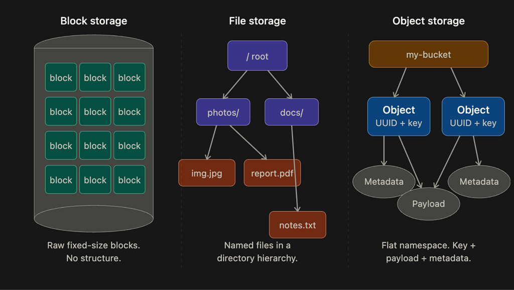
Block storage is the oldest and most low-level. When you plug a hard drive or SSD into a server, the operating system sees it as a sequence of raw blocks, each typically 4KB in size. The OS decides how to format those blocks and build a file system on top of them. Some applications, like databases and virtual machine engines, skip the file system entirely and manage the blocks directly, which gives them maximum control and performance.

Block storage doesn’t have to be physically attached. You can connect to block storage over a network using protocols like Fibre Channel or iSCSI. The server still sees raw blocks, as if the drive were directly attached, but the data sits somewhere else on the network. This is how cloud providers like AWS offer Elastic Block Store (EBS): you attach a network drive to your VM and it behaves like a local disk.

Block storage is fast and flexible, but it’s also expensive and doesn’t scale cheaply to petabytes.

File Storage

File storage is built on top of block storage. It adds a layer that handles the complexity of managing blocks and gives you a familiar directory hierarchy: folders, subfolders, and files. You don’t deal with blocks at all. You just read and write files using paths like /documents/report.pdf.

File storage becomes especially useful when multiple servers need to share the same files. Protocols like NFS and SMB/CIFS allow many machines to mount the same file share and read and write to it concurrently. This is how shared drives inside organizations typically work, and it’s how many legacy enterprise applications store data.

File storage is easier to use than block storage, but it still doesn’t scale to the level that object storage can. Hierarchical directory structures become slow and complex when you have billions of files.

Object Storage

Object storage is the newest of the three and the most different. It makes a deliberate tradeoff: give up performance and mutability in exchange for near-unlimited scalability, very high durability, and low cost.

There are no directories in object storage. Everything lives in a flat namespace inside containers called buckets. Every object is accessed via a RESTful HTTP API using a unique key. You can’t partially update an object. If you want to change a file, you replace the entire object or create a new version. This immutability constraint sounds limiting, but it’s actually what makes object storage so cheap to operate at scale, because it simplifies replication and consistency considerably.

AWS S3, Google Cloud Storage, and Azure Blob Storage are all object storage systems. They’re the foundation of most modern cloud architectures: video files, backups, data lake storage, machine learning datasets, static website assets, and more.

Comparison Table

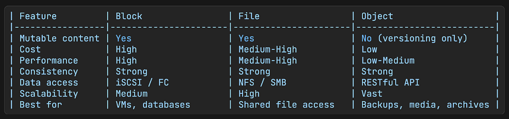
The key constraint to internalize: objects are immutable. You cannot edit part of an object. You replace the whole thing or you version it. This constraint is not an accident. It’s a deliberate design choice that enables the durability and scale properties that make object storage useful in the first place.

Key Terms

These are the concepts you need to know before we get into the design.

Bucket

A bucket is a logical container for objects. Think of it like a top-level folder, except it’s not really a folder since there’s no hierarchy inside it. Bucket names must be globally unique across all users of the system, not just within your account. You have to create a bucket before you can store anything in it.

Object

An object is an individual piece of data stored in a bucket. It has two parts. The payload is the actual data bytes, which can be anything: a photo, a video, a CSV file, a binary blob. The metadata is a set of key-value pairs that describe the object, things like content type, creation timestamp, custom tags, and anything else the application needs to store alongside the data. The metadata is stored separately from the payload and is much smaller.

Object Key

Every object is identified by a key, which is just a string. In S3, that key looks like a file path: photos/2024/vacation.jpg. But there are no actual directories. The entire string, slashes and all, is just the key. S3 lets you use slashes as a convention to simulate folders, but under the hood it’s still a flat namespace. This distinction matters when we design the listing feature later.

Versioning

Versioning is a bucket-level feature that keeps all previous versions of an object instead of overwriting them. When versioning is enabled, uploading an object with the same key as an existing object doesn’t replace it. It creates a new version alongside the old one. You can retrieve, restore, or delete any version at any time. This protects against accidental overwrites and deletions.

Durability SLA

The S3 Standard storage class is designed for 99.999999999% durability, which is called eleven nines. In practical terms, if you store 10 million objects for 10,000 years, you’d expect to lose one. That’s not an accident. It comes from specific engineering decisions around replication and error correction, which we’ll get into in the durability section.

Clarifying Requirements

Before touching any design, you need to understand what you’re actually building and at what scale. Candidates who skip this step in interviews fail immediately, because they end up designing the wrong thing at the wrong scale.

Questions to Ask

• What are the core operations? Upload, download, delete, list?
• Do we need versioning?
• How much data do we need to store in year one?
• What durability and availability targets do we need?
• Do we need to support large file uploads, like files that are multiple gigabytes?
• Any access control requirements? Do different users own different buckets?

Our Design Assumptions

For this design, we’ll assume:

• Core operations: bucket creation, object upload and download, object versioning, and listing objects in a bucket by prefix
• 100 petabytes of total data
• Durability target: six nines, which is 99.9999%
• Availability target: four nines, which is 99.99%
• Must handle both small objects (tens of kilobytes) and large objects (several gigabytes)

Now let’s figure out what these requirements actually mean for infrastructure.

Capacity Estimation

Math matters in system design because it tells you what kind of infrastructure you need. Vague statements like “we’ll need a distributed database” aren’t useful without numbers behind them. Let’s work through the estimates.

Object Size Distribution

In practice, object storage systems see a mix of object sizes. A reasonable assumption for a general-purpose system:

• 20% of objects are small, under 1MB, with a median size of about 0.5MB. These might be thumbnails, config files, or short documents.
• 60% of objects are medium-sized, between 1MB and 64MB, with a median of about 32MB. These might be images, audio files, or compressed datasets.
• 20% of objects are large, over 64MB, with a median of about 200MB. These might be videos, database backups, or large archives.

Total Object Count

We’re targeting 100 petabytes of stored data. In practice, storage systems don’t fill to capacity, so let’s assume 40% utilization, meaning we provision enough storage to hold 100PB when 40% full.

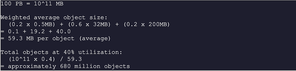
680 million objects is a lot. This tells us immediately that no single machine can store or index all of this. We need distributed storage and a distributed metadata index from day one.

Metadata Storage

Each object needs a metadata record. If we assume roughly 1KB per record (object name, bucket, timestamps, UUID, tags), then:

680GB of metadata is manageable in a database, but the access patterns will require sharding as we scale. The metadata store is separate from the data store, which we’ll cover in the design.

IOPS Constraints

A standard SATA hard drive spinning at 7200 RPM can handle roughly 100 to 150 random seeks per second. This is called IOPS, or input/output operations per second. At 680 million objects spread across many disks, the IOPS constraint becomes a real bottleneck, especially for small object workloads where you’re doing many small reads and writes rather than a few large sequential ones. This is one reason we’ll later choose to merge many small objects into a single larger file on disk, instead of storing each object as its own file.

Design Philosophy: Separating Metadata from Data

Before we look at the full architecture, there’s one core design principle that shapes everything else: the metadata and the data are stored separately, and for good reason.

This idea comes from how UNIX file systems work. In UNIX, when you save a file, the filename and the actual data bytes are not stored together. The filename and other file information (size, permissions, timestamps, disk location) live in a data structure called an inode. The actual data bytes live in separate disk blocks that the inode points to.

Object storage works the same way. The metadata store is like the inode layer. It holds the object name, bucket, size, and a UUID that points to where the actual bytes live. The data store is like the disk. It holds the raw bytes, and it only knows about UUIDs, not names or paths.

Why separate them? Because they have completely different characteristics. The data is immutable. Once written, it never changes. The metadata is mutable. You can update tags, rename objects (in some implementations), or add versioning records. They need different consistency guarantees, different storage engines, and different scaling strategies. Keeping them separate lets us optimize each independently.

High-Level Architecture

With that principle in mind, here’s how the full system is structured.

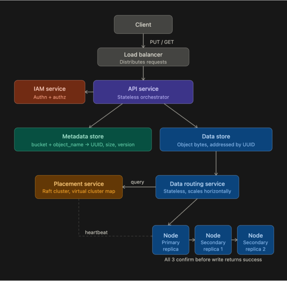
Components

Upload Flow

Let’s trace exactly what happens when a user uploads a file named report.pdf to a bucket called company-docs.

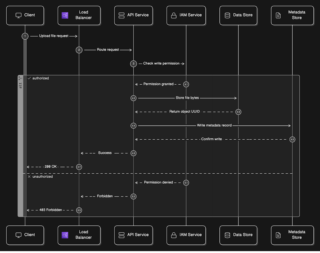
• The client sends a PUT /company-docs/report.pdf HTTP request with the file bytes in the request body.
• The request hits the load balancer and gets routed to one of the API service instances.
• The API service calls the IAM service to confirm the user has WRITE permission on the company-docs bucket. If not, the request is rejected immediately with a 403 Forbidden.
• The API service forwards the file bytes to the data store. The data store persists the bytes and returns a UUID, a unique identifier for this specific object.
• The API service writes a metadata record to the metadata store. This record contains the object name (report.pdf), the bucket ID, the UUID returned from the data store, the file size, the creation timestamp, and any metadata tags the user provided.
• A 200 OK response is returned to the client.

The metadata record now acts as the bridge between the human-readable path (company-docs/report.pdf) and the actual bytes stored by UUID in the data store.

Download Flow

Now let’s trace what happens when someone requests that same file.

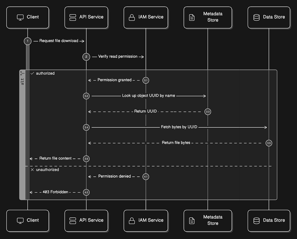
• The client sends a GET /company-docs/report.pdf request.
• The API service calls IAM to verify READ permission.
• The API service queries the metadata store: “what is the UUID for the object named report.pdf in the bucket company-docs?”
• The API service takes that UUID and fetches the actual bytes from the data store.
• The bytes are returned to the client.

Notice that the data store never knows the file was called report.pdf. From its perspective, someone asked for the object with a specific UUID and it returned the bytes. The translation from name to UUID always happens in the metadata store.

Deep Dive: Data Store

The data store is where most of the interesting engineering happens. Let’s break down its internal architecture.

Internal Components

Data Routing Service

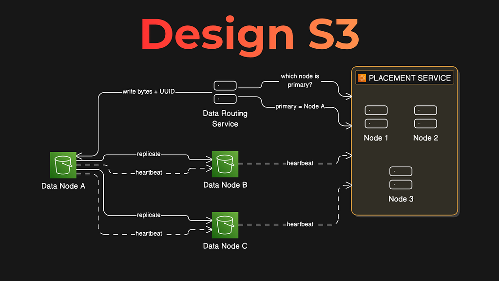
The data routing service is the entry point into the data store. It’s stateless, meaning it holds no state itself, so you can scale it horizontally by adding more instances. When a write comes in, it asks the placement service which data node should receive the data, then sends the data there. When a read comes in, it asks the placement service where the data lives, then fetches it.

Placement Service

The placement service is responsible for knowing the physical layout of the entire storage cluster. It maintains a virtual cluster map, which is essentially a registry of every data node, what rack it’s in, what availability zone it’s in, how many disks it has, and how much space is used on each disk.

The placement service continuously receives heartbeat messages from every data node. A heartbeat is a small message a node sends every few seconds saying “I’m alive, here’s my current state.” If the placement service doesn’t hear from a node within a configurable grace period (typically 15 seconds), it marks that node as down and stops sending new data to it.

Because the placement service is so critical, you run it as a cluster of 5 or 7 nodes using a consensus algorithm like Raft or Paxos. A consensus algorithm ensures the cluster agrees on a single consistent view of the world even if some nodes fail. With a 7-node cluster, you can lose 3 nodes simultaneously and the service keeps running. With a 5-node cluster, you can lose 2. You never run this as a single instance, because if it goes down, the entire storage cluster becomes unavailable for writes.

Data Nodes

Data nodes are where the actual bytes live. Each data node manages one or more physical disks. Each node runs a daemon process that sends heartbeats to the placement service with information about disk count and available space. When the placement service receives a heartbeat from a new node it hasn’t seen before, it assigns that node an ID, adds it to the virtual cluster map, and tells the node where to replicate data.

Data Persistence Flow

Here’s the step-by-step flow when a new object is written to the data store:

• The API service sends the object bytes to the data routing service.
• The data routing service generates a UUID for this object and asks the placement service: which data node should be primary for this object?
• The data routing service sends the bytes and the UUID to the primary data node.
• The primary data node saves the bytes locally and then replicates them to two secondary data nodes.
• The primary node sends a confirmation back to the data routing service only after all three nodes (primary plus two secondaries) have confirmed the write.
• The UUID is returned to the API service.

Step 5 is a critical design decision. By requiring all three nodes to confirm before returning a response, we get strong consistency: the data is guaranteed to be durable before the caller receives a success. The tradeoff is latency. The write is only as fast as the slowest of the three nodes.

You could choose weaker consistency: respond after just the primary writes, and let replication happen asynchronously in the background. That’s faster, but if the primary node crashes before replication finishes, you’ve lost data. For an object storage system whose core promise is durability, strong consistency is the right default.

How Data is Actually Stored on Disk

Here’s a design decision that seems minor but has major consequences at scale: how do you physically lay out objects on a data node’s disk?

The Naive Approach: One File Per Object

The most obvious approach is to store each object as its own file on the filesystem. You upload photo.jpg, and it becomes /data/photo.jpg on disk. Simple, intuitive, and completely wrong at scale.

Two things break down when you have millions of small objects stored as individual files:

Wasted disk blocks: File systems allocate space in fixed-size blocks, typically 4KB. If your object is 200 bytes, it still occupies an entire 4KB block on disk. With millions of small objects, you’re wasting a huge percentage of your storage capacity on empty space.

Inode exhaustion: An inode is a data structure the file system uses to track each file’s metadata: its size, location on disk, permissions, timestamps. Most file systems have a fixed number of inodes, set when the disk is initialized. With millions of files, you can run out of inodes even if you still have free disk space. When that happens, you can’t create new files, even though the disk isn’t full. The OS also struggles to manage large inode tables efficiently, even with aggressive caching.

The Solution: Merge Small Objects into Large Files

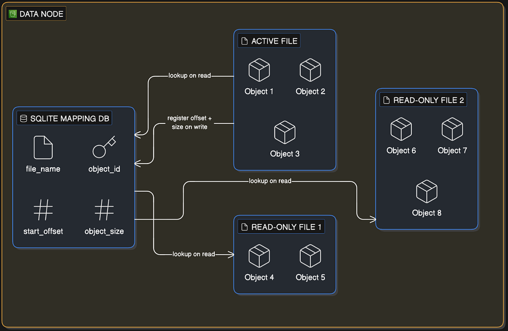
The fix is to merge many small objects into a single large file, similar to how a write-ahead log works in a database. Here’s how it works:

• Each data node maintains one active read-write file. New objects are appended to the end of this file, one after another, sequentially.
• When the active file reaches a size threshold (typically a few gigabytes), it gets marked as read-only and a new active file is opened.
• Read-only files only serve read requests. The active file takes all new writes.
• To avoid a write throughput bottleneck on multi-core servers, each CPU core gets its own active read-write file. This lets cores write in parallel without waiting for each other.

Now, how do you find a specific object inside one of these large merged files? You need an index. Each data node maintains a local SQLite database with a mapping table:

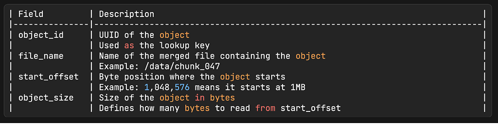
To read an object: look up its UUID in the mapping table, open the file at file_name, seek to start_offset, read object_size bytes. It’s fast, deterministic, and doesn’t require scanning anything.

Why SQLite specifically? The access pattern here is write-once, read-many. SQLite uses a B+ tree storage engine, which is faster for reads than write-optimized alternatives like RocksDB. Since each data node has its own isolated mapping table, there’s no need for a distributed database. SQLite running locally on each node is the right tool.

Chunking Large Objects for Parallel Reads

We’ve talked about merging small objects into large files to solve the inode problem. Large objects have the opposite problem: they’re too big to read efficiently from a single disk in a single sequential stream.

The solution is chunking. When a large object is stored, the data store splits it into fixed-size chunks (typically 64MB to 128MB each) and distributes those chunks across multiple data nodes. The object’s metadata record stores the list of chunk locations in order.

When a client downloads the large object, the data store fetches all chunks in parallel from their respective nodes and streams them back in sequence. Instead of being limited to the read throughput of one disk, you’re reading from many disks simultaneously. A 1GB object split into 8 chunks across 8 nodes reads roughly 8x faster than a single sequential read.

This also maps cleanly onto erasure coding. With (8+4) erasure coding, the data is already split into 8 data chunks stored on 8 nodes. Reading those chunks in parallel is the natural access pattern, not an exception.

Range Requests for Large Files

Chunking enables another important capability: range requests. The HTTP Range header allows a client to request a specific byte range within an object rather than the whole thing.

A request like Range: bytes=52428800–104857599 asks for bytes 50MB through 100MB of the object. The data store looks at the chunk layout, figures out which chunks contain those bytes, fetches only those chunks, and returns just the requested range.

This matters enormously for video. When you scrub to the middle of a 2GB video file, the player doesn’t download the whole file from the beginning. It sends a range request for the bytes starting at that timestamp and streams from there. Without range request support, video scrubbing would be unusable.

The same pattern applies to resumable downloads. If a large file download fails halfway through, the client can resume from where it stopped by sending a range request starting at the last received byte, rather than re-downloading from zero.

Durability

Durability is the central promise of object storage. Six nines (99.9999%) means that if you store 1 million objects for 1,000 years, you’d expect to lose one. Here’s how you actually achieve that.

Replication

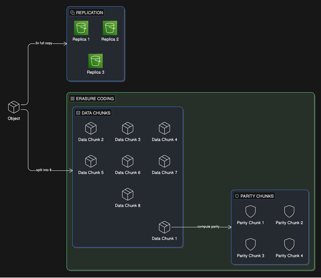
The baseline strategy is to replicate every object to multiple data nodes in different physical locations. Here’s why three copies specifically, and why failure domains matter.

Why Three Copies

A modern spinning hard drive has an annual failure rate of roughly 0.81%, based on data published by Backblaze from their large-scale storage systems. If you store one copy of your data on one drive, you have a 0.81% chance of losing it in any given year. That’s terrible.

With three independent copies on three different drives:

That’s the math behind the six nines target. Three independent copies on independently-failing hardware gets you there.

Failure Domains

Raw math assumes the three drives fail independently. In reality, hardware doesn’t always fail independently. Physical failures often have a scope: they affect everything in a shared failure domain.

A failure domain is any group of hardware that shares a single point of failure. A server is a failure domain because it shares a power supply, motherboard, and network connection. A rack is a failure domain because it shares a network switch and a power distribution unit. An availability zone (a physically separate section of a data center with its own power and cooling) is a failure domain because a large-scale outage (flooding, fire, power grid failure) could take it down.

If you put all three copies of an object on drives in the same rack, and the rack’s power distribution unit fails, you’ve lost all three copies simultaneously. The math breaks down because the failures weren’t independent.

The solution is to place replicas in separate failure domains: different racks at minimum, different availability zones for important data, potentially different regions for disaster recovery. The placement service’s virtual cluster map contains the physical location of every node specifically so it can make this call when deciding where to put replicas.

Erasure Coding

Three-copy replication gives you six nines of durability with 200% storage overhead. You’re storing 3x the data you actually have. For a 100PB system, that means 300PB of physical storage for 100PB of actual data. At the cost of storage, that’s extremely expensive.

Erasure coding is an alternative that achieves better durability at much lower storage overhead, at the cost of more computation and complexity.

How Erasure Coding Works

Erasure coding breaks an object’s data into chunks and computes additional parity chunks using mathematics. A common configuration is called (8+4): split the data into 8 equal chunks, then compute 4 parity chunks, for 12 total. Each chunk is stored on a different data node in a different failure domain.

The mathematics of erasure coding guarantee that as long as any 8 of the 12 chunks are available, you can reconstruct the full original object. You can lose any 4 nodes simultaneously, in any combination, and lose nothing. The parity chunks are computed using Reed-Solomon error correction, the same mathematics used to protect data on CDs and DVDs.

The durability with (8+4) erasure coding works out to approximately 11 nines, significantly better than replication’s 6 nines, according to Backblaze’s calculations on their storage fleet.

Erasure Coding vs. Replication

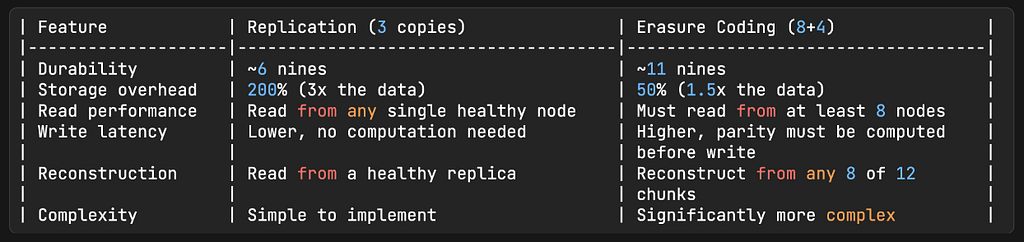
The practical rule: use replication when latency matters and your data volume is manageable. Use erasure coding when storage cost is the dominant concern and you’re operating at a scale where paying for 200% overhead is genuinely painful. For a 100PB object storage system, erasure coding can save you 150PB of physical storage. At cloud storage pricing, that’s tens of millions of dollars per year.

Checksum Verification

Even with replication or erasure coding protecting against node failures, there’s a third failure mode that’s easier to miss: silent data corruption.

Disk hardware can silently flip bits. Memory can corrupt data in transit between components. Network transmission can introduce errors. These corruptions don’t announce themselves. The hardware doesn’t raise an error. The data just quietly becomes wrong.

The standard defense is checksums. A checksum is a short value computed from the data using a function like MD5 or SHA-1. The key property of a good checksum function is that even a single flipped bit in the input produces a completely different checksum output. If you store the checksum alongside the data and recompute it on every read, you’ll immediately detect any corruption.

In our data store, each object gets its checksum appended when it’s written. The checksum is also computed for the entire merged file when that file is marked read-only. On every read, the system computes the checksum of the retrieved bytes and compares it to the stored checksum. If they don’t match, the system knows the data is corrupted and fetches it from another replica or reconstructs it from erasure coding chunks instead.

How S3 Transmits Checksums

There’s a subtle engineering detail worth understanding here. The naive approach to checksums on upload is: compute the checksum first, include it in the request header, then send the data. The problem is that you have to read the entire file twice: once to compute the checksum, and once to stream it in the upload.

S3 solves this using the HTTP Trailer header. Instead of putting the checksum at the start of the request, S3 appends it at the end of the data stream after the last byte has been sent. The client streams the data while computing the checksum in parallel, then appends it when the stream closes. One pass through the data instead of two. At S3’s scale, this matters: they compute around 4 billion checksums per second across the entire fleet.

Bracketing: Verifying Before Confirming

S3 does one more thing before returning a success response that most storage systems skip: bracketing. After erasure coding and storing all shards, and before sending 200 OK back to the client, S3 reverses the entire transformation. It takes the stored shards, reconstructs the original object from them, and verifies the result matches what was uploaded.

This is more expensive than just storing the data, but it catches a class of bugs that checksums alone won’t catch: cases where the erasure coding itself introduced an error, or where the shards were stored in the wrong order. If the reconstruction fails, the write is rejected and the client is told to retry. The cost is extra latency on every write. The benefit is that a successful response from S3 means the data is not just stored, but provably recoverable.

Failure Recovery and Re-replication

Checksums tell you when data is corrupted. Heartbeats tell you when a node is down. But detecting a problem is only half the job. The other half is fixing it fast enough that you don’t accumulate risk.

What Happens When a Node Goes Down

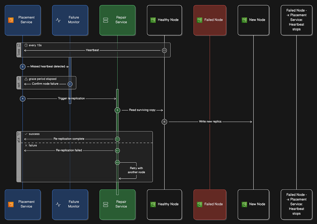
When the placement service stops receiving heartbeats from a data node, it doesn’t immediately start re-replicating. Most node failures are transient: a brief network partition, a server reboot, a firmware update. If you start aggressively re-replicating every time a node misses a few heartbeats, you’ll waste enormous bandwidth moving data for nodes that come back online in 5 minutes.

So systems typically wait a grace period of 15 to 30 minutes before treating a node as truly failed and initiating re-replication. During that window the affected objects are under-replicated: you have fewer copies than your durability target requires. The system is more vulnerable during this time, which is why keeping the grace period short matters.

Once a node is confirmed failed, the placement service identifies every object that had a replica or erasure coding chunk on that node. For each one, it selects a healthy destination node and instructs other nodes holding the remaining copies to replicate to it. This happens in parallel across all affected objects.

Scaling Repair to Match Failure Rate

Hardware failure rates aren’t constant. They spike during extreme weather, power events, and when a batch of drives from the same manufacturing run all hit the same age-related failure mode simultaneously. A fixed-capacity repair service gets overwhelmed during these spikes.

S3 runs a separate monitoring service that tracks the current failure rate and dynamically scales the repair service to match. When failures are rare, the repair service runs at low capacity. When a failure spike hits, it scales up aggressively to keep re-replication pace with the rate of data going under-replicated. Nodes also keep a reserved pool of free storage specifically for absorbing incoming replicas during recovery, so many nodes can participate in parallel rather than bottlenecking on a few.

Periodic Data Audits

Beyond responding to failures, S3 runs continuous background audits. Background processes scan stored objects, recompute checksums against stored shards, and flag anything that doesn’t match. This catches silent corruption on drives that are still “alive” from a heartbeat perspective but have degraded sectors that silently return wrong bytes. When a bad sector is found, the affected shard is reconstructed from other nodes and rewritten to a healthy location.

Metadata Data Model

The metadata store is a relational database. Its job is to answer three types of queries efficiently:

• Find the object ID (UUID) by object name and bucket. This happens on every upload and download.
• Insert or delete an object record by name. This happens on every upload and delete operation.
• List all objects in a bucket whose names start with a given prefix. This is the listing feature, which we’ll cover in detail.

Schema Design

The schema has two tables. The bucket table stores information about buckets, and the object table stores information about individual objects.

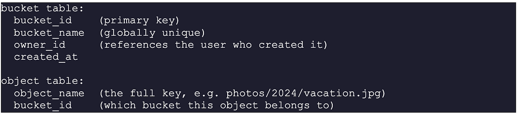
The relationship between a bucket and its objects is a standard one-to-many: one bucket contains many objects. The object_id UUID is the link between the metadata store and the data store.

Scaling the Bucket Table

Bucket counts are naturally bounded. Most systems limit how many buckets a user can create, and even at 1 million users with 10 buckets each, you have only 10 million bucket records. At 1KB per record, that’s 10GB total. A single well-tuned database server can handle this easily. If read volume is high, add read replicas to distribute the load.

Scaling the Object Table

The object table is where scale becomes a real challenge. At 680 million objects with 1KB per record, that’s 680GB of data just for the metadata. A single database instance can hold this, but it won’t handle the query volume at our scale. We need to shard the table, meaning split it across multiple database instances, each holding a subset of the rows.

Sharding introduces a key question: what do we use as the sharding key? The sharding key determines which rows land on which database instance, and it needs to distribute data evenly while also keeping related queries on the same shard.

Option 1: Shard by bucket_id

All objects from the same bucket land on the same shard. This seems logical, but it fails badly for large buckets. A bucket with 10 billion objects would create a single massively overloaded shard while others sit mostly empty. These are called hot shards, and they defeat the purpose of sharding.

Option 2: Shard by object_id

Shard by the UUID of each object. This distributes data perfectly evenly, but it breaks our most common queries. Looking up an object by its name requires checking every shard, because you don’t know which shard has the right UUID until you find the name. That’s an expensive scatter-gather operation on every read.

Option 3: Shard by hash of (bucket_name, object_name)

This is the right choice. Hash the combination of the bucket name and object name, and use that hash value to determine the shard. Because most operations (lookups, inserts, deletes) are keyed on the object’s name, a given name always hashes to the same shard. You can route any name-based query directly to the correct shard without a broadcast.

Even distribution is maintained because hash functions spread values uniformly across the available shards. And the combination of bucket_name and object_name handles the case where the same filename exists in different buckets: they hash to different values and land on different shards, which is correct behavior.

The Co-location Tradeoff

Hashing by (bucket_name, object_name) scatters objects from the same bucket across many shards. This is good for write throughput: uploads to the same bucket don’t all funnel to the same database instance. But it has a cost: objects that are logically related (same bucket, similar prefix) land on completely different shards with no guarantee of physical proximity.

Some systems partition first by account ID, then hash within the account. This co-locates all of a given user’s data on a predictable subset of shards, which makes account-level operations like quota checks, billing, and access audits faster. The tradeoff is that large accounts with billions of objects become hot spots. Neither approach is strictly better. It depends on whether your dominant query pattern is per-object lookups (hash wins) or account-level aggregation (account-first partitioning wins).

Listing Objects in a Bucket

The listing operation is one of the trickier parts of object storage design, and it’s worth understanding in depth because it’s a common interview topic.

How Prefixes Work

S3 doesn’t have real directories, but it uses a concept called prefixes to simulate them. A prefix is just the beginning of an object’s key. If you list a bucket with the prefix photos/2024/, you get back all objects whose key starts with those characters, regardless of what comes after. If an object exists with the key photos/2024/vacation.jpg, it would appear in the results. An object with the key photos/2023/birthday.jpg would not.

S3 also supports a delimiter parameter (usually /), which causes objects to be “rolled up” at each delimiter boundary. If you list with prefix photos/ and delimiter /, you won’t see photos/2024/vacation.jpg individually. Instead, you’ll see photos/2024/ as a common prefix, as if it were a folder. This is how S3 clients like the AWS console simulate a folder browsing experience even though the underlying storage is flat.

Listing with a Single Database

With a single unsharded database, listing is a straightforward SQL query:

The LIKE clause matches all object names that start with the given prefix. The ORDER BY gives you consistent alphabetical ordering across pages. The LIMIT prevents accidentally returning billions of rows in a single response. Pagination is handled by the client sending a cursor (the last key it received) with each subsequent request, and the server querying for names greater than that cursor.

Listing with a Sharded Database

With a sharded metadata database, listing gets significantly harder. The objects matching a given prefix are scattered across many shards, because they were distributed by hashing their names. You don’t know which shards contain matching objects without querying all of them.

The naive approach is a scatter-gather query: send the listing query to every shard in parallel, collect all results, merge and sort them in the application layer, then return the page to the client. This works but has real costs. Every listing operation hits all shards. Implementing cursor-based pagination is complicated because each shard has its own position in the result set.

The practical solution used in production object storage systems is denormalization. You maintain a separate listing table sharded by bucket_id. This table contains only the data needed for listing: the bucket ID and the object names within it. When an object is created or deleted, both the main object table and the listing table are updated. Because the listing table is sharded by bucket_id, a single listing query only needs to hit the shards that hold that bucket’s data, rather than all shards.

This approach involves some added write complexity and the extra storage for the listing table, but it’s the right tradeoff. Object listing is explicitly a secondary use case in object storage. AWS, Google, and Azure all document that listing performance is limited, and their APIs reflect this with response sizes capped at 1,000 objects per request and mandatory pagination for larger results.

Object Versioning

Versioning is the feature that protects users from accidental overwrites and deletions. It’s enabled at the bucket level and changes how uploads and deletes work.

How Versioning Changes Uploads

Without versioning: uploading a file with the same key as an existing object replaces the metadata record. The old object bytes get marked for deletion.

With versioning: uploading a file with the same key creates a new metadata record alongside the old one. Both records exist simultaneously. The object table gets two additional columns:

object_version: A TIMEUUID (a UUID that encodes the timestamp at which it was created) generated at insert time. Because TIMEUUIDs encode timestamps, you can always determine which version is most recent by finding the one with the largest TIMEUUID value for a given object name.

is_delete_marker: A boolean flag used when an object is deleted in a versioned bucket. More on this below.

When a client requests an object without specifying a version, the system returns the version with the largest TIMEUUID, which is the most recently created version.

How Versioning Changes Deletes

In a non-versioned bucket, deleting an object removes its metadata record and marks the bytes for garbage collection. In a versioned bucket, deletion doesn’t remove anything immediately.

Instead, the system inserts a new record for that object with is_delete_marker set to true. This delete marker becomes the current version (it has the newest TIMEUUID). When a client tries to GET the object, the system finds the current version is a delete marker and returns a 404 Not Found response, as if the object doesn’t exist. But all the previous versions are still there in the metadata table, and their bytes are still in the data store.

To permanently delete a versioned object, you must explicitly delete a specific version by its version ID. To restore a deleted object, you can either delete the delete marker (which reveals the most recent real version underneath) or copy an old version back as a new upload.

Large File Uploads: Multipart Upload

Uploading a 5GB file as a single HTTP request creates a reliability problem. HTTP connections can drop. Networks have transient failures. If you’re uploading a 5GB file and the connection breaks at 99% completion, you have to start over from zero. For large files, this becomes genuinely painful.

Multipart upload solves this by splitting large files into independently-uploadable pieces.

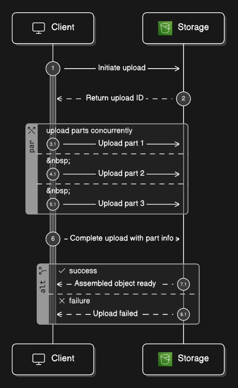
The Process

• The client sends an initiation request to the data store. The data store responds with an uploadID, a unique identifier for this specific multipart upload session.
• The client splits the file into parts. Part sizes typically range from 5MB to 200MB each. Each part is uploaded as a separate HTTP request, with the uploadID attached to identify which session it belongs to.
• As each part is successfully received and stored, the data store returns an ETag for that part. An ETag is the MD5 checksum of the part’s bytes. The client stores these ETags.
• After all parts are uploaded, the client sends a completion request containing the uploadID, the list of part numbers in order, and all the ETags.
• The data store verifies the ETags, reassembles the parts in the specified order into the final object, and returns a success response. For very large files, this reassembly can take several minutes.

The key advantage is that if any individual part fails, only that part needs to be re-uploaded. The rest are already saved. You can also upload multiple parts in parallel, using multiple simultaneous connections to maximize bandwidth utilization.

The downside: after the object is reassembled from its parts, the individual part files are orphaned. They take up space but are no longer needed. The garbage collector handles their cleanup.

Why ETags Matter

The ETag serves two purposes. First, it’s a checksum that lets the data store verify each part arrived uncorrupted. Second, when the client sends ETags in the completion request, the data store can verify that it actually received the parts the client claims to have uploaded, in the right order, before assembling the final object. This prevents assembling a corrupt or incomplete file.

Garbage Collection

Over time, the data store accumulates bytes that are no longer referenced by any live object. If you don’t clean these up, you waste disk space. The garbage collector is the background process responsible for reclaiming this space.

What Becomes Garbage

Lazily deleted objects: When an object is deleted, the metadata record is removed (or replaced with a delete marker in versioned buckets), but the bytes on disk are not immediately freed. Immediate deletion would add latency to the delete operation and complicate the data store’s append-only write model. Instead, bytes are left on disk and cleaned up later.

Orphaned multipart parts: After a multipart upload completes and the object is assembled, the individual part files are no longer needed. If a multipart upload is abandoned without completing (for example, a client crashes mid-upload), the parts are never assembled and never cleaned up by the completion path. The garbage collector finds and removes them.

Corrupted data: Objects that fail checksum verification during reads are flagged as corrupted. The data has already been reconstructed from a clean replica, so the corrupted copy can be safely discarded.

How Compaction Works

The garbage collector uses a compaction process to clean up data node files. Here’s the step-by-step:

• The garbage collector identifies read-only data files that contain a significant number of deleted or corrupted objects.
• It creates a new output file and scans the old file from beginning to end.
• For each object in the old file, it checks the object_mapping table to see if the object is still live (not deleted, not corrupted).
• Live objects are copied into the new output file. Deleted or corrupted objects are skipped.
• Once all live objects are copied, the object_mapping table is updated in a single database transaction, changing the file_name and start_offset for every moved object to their new locations in the output file.
• The old file is deleted.

The transaction in step 5 is important. It ensures that the mapping table and the on-disk layout are always consistent. If the garbage collector crashes between step 4 and step 5, the old file still exists and the mapping still points to it. Nothing is lost. If the crash happens after step 5, the new layout is in place and the old file can be deleted safely on restart.

To avoid creating many small compacted files, the garbage collector batches its work. It waits until it has identified a large number of read-only files to process, then compacts them all into a small number of large new files. For replicated data, the garbage collector runs independently on each replica node. For erasure-coded data with an (8+4) configuration, it runs on all 12 chunk nodes.

Storage Tiers and Lifecycle Policies

Not all data needs to be equally fast or equally expensive to store. A video uploaded this morning needs to be retrievable in milliseconds. An audit log from three years ago might be fine to wait 12 hours for. Treating both the same way wastes a lot of money.

Object storage systems solve this with storage tiers: different classes of storage with different cost and latency profiles, and lifecycle policies that move objects between tiers automatically based on rules you define.

Storage Tiers

Hot Storage

Hot storage is optimized for frequent access and low latency. Data is stored on fast drives, often with replication tuned for quick reads. First-byte latency is in the single-digit milliseconds. It’s the most expensive tier and is the right choice for objects that users actively read: profile photos, product images, recently uploaded files, application assets.

Cool Storage

Cool storage trades some read performance for lower cost. Data is stored on slower spinning disks with slightly relaxed read SLAs, typically first-byte latency in the range of seconds rather than milliseconds. Cost per GB is significantly lower than hot storage. The right choice for data that’s accessed occasionally but not frequently, like monthly reports, logs from the past few months, or backups you might need to restore from.

Archive Storage

Archive storage is designed for data you almost never read but legally or operationally must keep. Retrieval times can range from minutes to hours because the data may be stored on tape or in extremely low-power disk systems that need to spin up before serving a request. Cost per GB is the lowest of any tier by a large margin. The right choice for compliance archives, old database backups, or historical records you need to retain for years but rarely touch.

AWS Glacier is Amazon’s archive tier. Azure Archive and Google Coldline serve the same purpose on their platforms.

Lifecycle Policies

Lifecycle policies are rules you attach to a bucket that automatically move objects between storage tiers based on age or access patterns. You define them once and the storage system handles the transitions.

A typical policy might look like: keep objects in hot storage for the first 30 days, move to cool storage after 30 days, move to archive after 90 days, and permanently delete after 7 years. This maps naturally to how real data ages: it’s accessed often right after creation, less often after a few weeks, rarely after a few months, and almost never after a year or two.

Lifecycle policies matter for system design because they directly affect your storage cost calculation. A system that keeps everything in hot storage forever is orders of magnitude more expensive than one with intelligent tiering. For a 100PB system where most data is over a year old, the difference between hot-only and tiered storage can be 10x or more in monthly cost.

At the architecture level, implementing tiers means the metadata store needs a storage_class field on each object record, and a background service that periodically scans for objects matching lifecycle rule criteria and moves them. Moving an object between tiers doesn’t change its key or UUID. From the user’s perspective, the object is still at the same path. The only difference is how long it takes to retrieve.

Monitoring and Observability

A storage system at this scale has thousands of moving parts. Drives fail. Nodes go down. Replication falls behind. Garbage collection stalls. Without visibility into what’s happening, you’re operating blind.

This section is intentionally brief because monitoring is not what makes object storage design interesting. But it’s worth naming the signals that matter specifically for this kind of system.

Key Metrics to Track

Replication lag: How many objects are currently under-replicated, meaning they have fewer copies than the durability target requires. This is your real-time durability risk indicator. If this number spikes, you either have a node failure in progress or your repair service is falling behind.

Checksum failure rate: How many reads per second are returning corrupted data that requires reconstruction from another replica. A sudden spike here points to a drive with bad sectors or a network component introducing bit flips.

Data node heartbeat status: Which nodes are currently marked as down or degraded by the placement service. This is your operational dashboard for cluster health.

Write and read latency percentiles: Track p50, p95, and p99 latencies separately. The p99 is what your worst-affected users experience. A rising p99 with a stable p50 usually means a specific slow node is dragging tail latency up without affecting the median.

Garbage collection backlog: How much storage space is occupied by deleted objects waiting to be compacted. If this grows indefinitely, your GC process is not keeping pace with deletes.

Storage utilization per node: How full each data node is. The placement service uses this to avoid routing new writes to nearly-full nodes, but you need to see it yourself to know when to add capacity.

Alerting Thresholds

The metrics above are only useful if someone acts on them. A few thresholds worth alerting on:

• Under-replicated object count exceeds zero for more than 30 minutes (node failure in progress, repair not keeping up)
• Checksum failure rate rises above your baseline by more than 2x (potential drive degradation)
• Any data node stops sending heartbeats for more than 15 seconds (possible node failure)
• Storage utilization on any node exceeds 80% (capacity planning signal, not an emergency yet)
• GC backlog grows for more than 24 hours without shrinking (GC process stalled or overwhelmed)

Monitoring doesn’t change the design, but it’s what turns a system that works in theory into one you can actually operate at scale without being surprised by failures that were building up for days.

Trade-Offs Summary

Every major decision in this design involves a real tradeoff. Let’s be explicit about what each one is.

Strong Consistency vs. Latency on Writes

We chose to require all three replicas to confirm a write before returning success to the client. This gives strong consistency: the data is guaranteed to be durable before the caller gets a response. The cost is write latency, because you’re waiting for the slowest of the three replicas on every write.

The alternative is eventual consistency: respond after just the primary node writes, and replicate asynchronously. Writes are faster, but if the primary fails before replication completes, you’ve permanently lost data. For an object storage system whose core value proposition is durability, this tradeoff isn’t worth it.

Replication vs. Erasure Coding

Three-copy replication is simple to implement and fast for both reads and writes. Erasure coding (8+4) achieves better durability (11 nines vs. 6 nines) and 75% lower storage overhead, but requires reading from 8 nodes on every read and computing parity on every write. It’s significantly more complex to implement and debug.

The right choice depends on your scale. At small scale, the simplicity of replication outweighs the cost savings from erasure coding. At hundreds of petabytes, the storage savings from erasure coding can be worth tens of millions of dollars annually, and the engineering investment to implement it correctly starts to pay for itself.

File-Per-Object vs. Merged Files

Storing each object as its own file is simple and intuitive. Merging objects into large files is more complex (you need the mapping table and the compaction process) but eliminates both inode exhaustion and wasted disk blocks for small objects. At 680 million objects, the merged file approach is necessary. At a thousand objects, it’s unnecessary complexity.

Listing Performance

Object storage doesn’t promise fast listing. The flat namespace combined with distributed sharding makes fast prefix scans inherently expensive. The denormalized listing table mitigates this but adds write overhead and storage cost. This is a known and accepted limitation of the architecture. Every major cloud object storage provider documents it and designs their APIs around it, with mandatory pagination and rate limits on list operations.

Metadata Sharding Key

Sharding by bucket_id creates hot shards for large buckets. Sharding by object_id breaks name-based lookups. Sharding by the hash of (bucket_name, object_name) gives even distribution while preserving the ability to route name-based queries to a single shard. It’s the right choice for this workload but comes with the caveat that cross-bucket queries become expensive scatter-gather operations, and account-level aggregation requires querying all shards.

Grace Period Before Re-replication

Waiting 15 to 30 minutes before re-replicating after a node failure avoids wasting bandwidth on transient failures, but it leaves objects under-replicated during that window. The right grace period depends on your observed ratio of transient to permanent failures. If most node disappearances are brief reboots, a longer grace period saves bandwidth. If most are real failures, a shorter period reduces your durability risk window.

Storage Tier Transitions

Moving objects to cheaper storage tiers reduces cost but increases retrieval latency. The right tier boundaries depend on your access pattern data. If you set the archive threshold too early, users who occasionally access older objects will experience multi-hour retrieval times and complain. If you set it too late, you’re overpaying for hot storage. Good lifecycle policy design requires measuring actual access patterns, not guessing.

Conclusion

Designing S3-like object storage at 100PB scale requires confronting problems you don’t encounter in typical web applications. A single database can’t store the metadata. A single server can’t hold the data. A naive file-per-object layout breaks at millions of objects. A single-copy storage system loses data as hardware fails. Every assumption you’d make for a small system breaks down.

The decisions that make the design work at scale:

• Separate the metadata store from the data store. They have different mutability, different consistency requirements, and different scaling strategies. Mixing them together would make both harder to optimize.
• Merge small objects into large files on disk. This avoids inode exhaustion and disk block waste, which are real operational problems that take down storage nodes if you ignore them.
• Chunk large objects and read them in parallel. A single disk’s throughput caps out quickly. Distributing a large object across many nodes and reading all chunks simultaneously is how you get fast reads at scale.
• Support range requests. Video scrubbing, resumable downloads, and partial reads all depend on being able to fetch a specific byte range without downloading the entire object.
• Replicate data across separate failure domains. Three copies in the same rack doesn’t give you three independent failure probabilities. Physical placement of replicas matters as much as the number of replicas.
• Use erasure coding when storage cost dominates. At 100PB, the difference between 200% overhead (replication) and 50% overhead (erasure coding) is 150PB of physical storage. That’s a real cost.
• Verify data end-to-end, not just at write time. Checksums on individual objects catch corruption, but bracketing (reconstructing and verifying before confirming a write) catches a broader class of bugs.
• Scale repair to match failure rate. A fixed-capacity repair service gets overwhelmed during failure spikes. Monitor the failure rate and scale repair capacity dynamically.
• Shard the metadata table by hash of (bucket_name, object_name). Sharding by bucket_id creates hot shards. Sharding by object_id breaks lookups. The hash approach handles both problems.
• Accept slow listing and design around it. Denormalize a separate listing table, paginate all responses, and document the limitation clearly.
• Use storage tiers and lifecycle policies. Keeping everything in hot storage forever is the most expensive possible configuration. Most data ages out of frequent access quickly; let the system move it automatically.
• Run garbage collection asynchronously. Immediate deletion adds latency to delete operations and complicates the append-only write model. Background compaction is slower but doesn’t block the critical path.

In an interview, what separates strong answers is the ability to explain the why behind each decision, not just name the components. Not just “we shard the metadata table” but “we shard by the name hash specifically because most operations are name-based lookups, and sharding by bucket_id creates hot shards for large buckets.” Not just “we use erasure coding” but “we use erasure coding because at 100PB, the 150PB of storage we save from the reduced overhead justifies the added read complexity and implementation cost.”

The deeper principle: object storage makes a deliberate bet. It gives up mutability, gives up fast listing, and gives up low write latency to achieve near-unlimited scale, very high durability, and low storage cost. Every design decision in this article follows from that bet. Understand the bet, and the entire design makes sense.

Design S3 Object Storage Like a Senior Engineer was originally published in Level Up Coding on Medium, where people are continuing the conversation by highlighting and responding to this story.