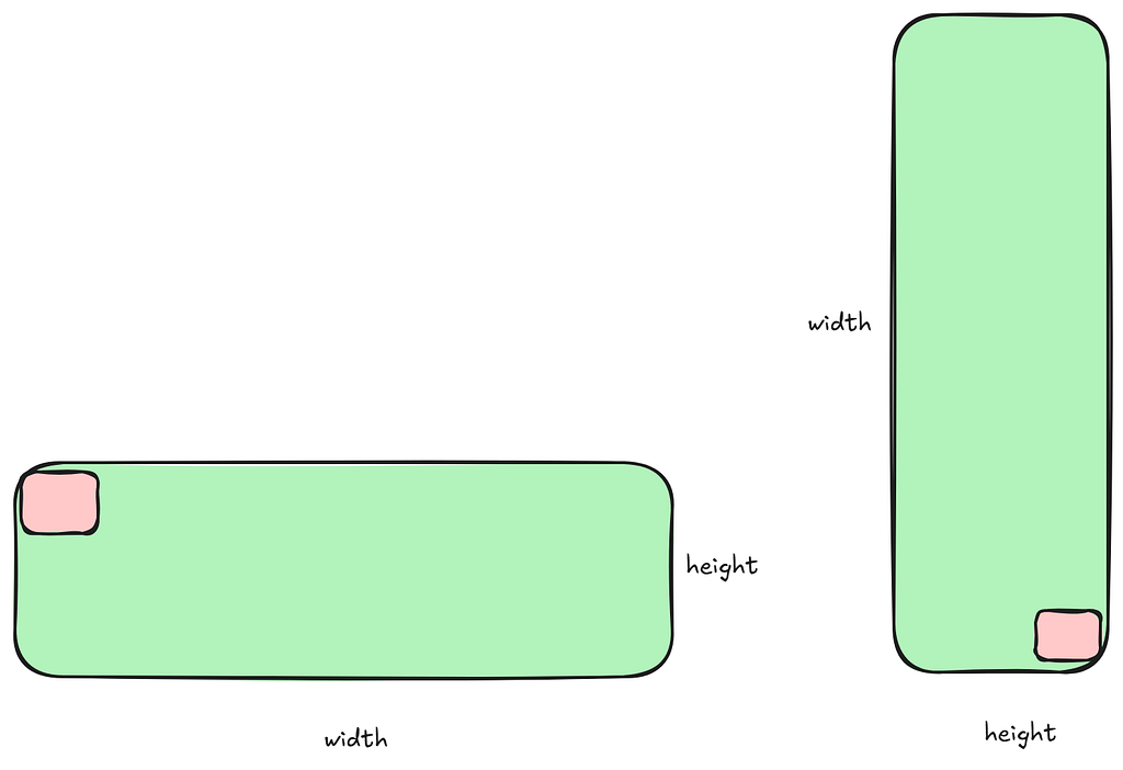
Matrix transpose is one of the most fundamental operations in deep learning and high-performance computing. The deceptively simple coordinate swap B[y][x]=A[x][y] may be just a double loop on the CPU, but on a throughput-oriented GPU architecture, the memory access pattern often matters far more than the compute logic itself. Writing an efficient transpose kernel is a classic litmus test for a CUDA engineer’s skills.
This article walks through a real CUDA implementation step by step — from the most naive version, evolving into efficient variants that combine Shared Memory, Bank-Conflict-Free Padding, and XOR Swizzle. Along the way, we’ll explain why shared memory bank conflicts arise and how a simple swizzle mechanism eliminates them.
The complete source code for all kernels and performance benchmarks discussed in this post is available in my open-source practice project: WingEdge777/Vitamin-CUDA
0. Why Is Transpose Hard? Coalesced vs. Non-Coalesced Access
In GPU global memory, the optimal access pattern is coalesced access. In short, when 32 threads in a warp access contiguous memory addresses, the GPU can merge these into very few memory transactions.
Matrix transpose has a fundamental tension:
- If we read by rows (coalesced reads), the transposed write must be by columns (non-coalesced, strided writes).
- If we read by columns (non-coalesced reads), the transposed write is by rows (coalesced writes), but the read side is now slow.
1. Naive Implementation
We implement two baseline versions — one prioritizing coalesced reads, the other coalesced writes:
- transpose_coalesced_read_kernel: Coalesced read, strided write.
- transpose_coalesced_write_kernel: Strided read, coalesced write.
const int naive_tiling_size = 16;

// naive coalesced read transpose
__global__ void transpose_coalesced_read_kernel(float *a, float *b, int width, int height) {
    int x = blockIdx.x * blockDim.x + threadIdx.x;
    int y = blockIdx.y * blockDim.y + threadIdx.y;
    if (x < width && y < height) {
        b[x * height + y] = a[y * width + x];
    }
}
// launch code
void transpose_coalesced_read(torch::Tensor a, torch::Tensor b) {
    CHECK_T(a);
    CHECK_T(b);
    cudaStream_t stream = at::cuda::getCurrentCUDAStream();
    const int height = a.size(0);
    const int width = a.size(1);
    const dim3 threads_per_block(naive_tiling_size, naive_tiling_size);
    const dim3 blocks_per_grid((width + naive_tiling_size - 1) / naive_tiling_size,
                               (height + naive_tiling_size - 1) / naive_tiling_size);
    transpose_coalesced_read_kernel<<<blocks_per_grid, threads_per_block, 0, stream>>>(
        a.data_ptr<float>(), b.data_ptr<float>(), width, height);
}
// naive coalesced write transpose
__global__ void transpose_coalesced_write_kernel(float *a, float *b, int width, int height) {
    int x = blockIdx.x * blockDim.x + threadIdx.x;
    int y = blockIdx.y * blockDim.y + threadIdx.y;
    if (x < height && y < width) {
        b[y * height + x] = a[x * width + y];
    }
}
void transpose_coalesced_write(torch::Tensor a, torch::Tensor b) {
    CHECK_T(a);
    CHECK_T(b);
    cudaStream_t stream = at::cuda::getCurrentCUDAStream();
    const int height = a.size(0);
    const int width = a.size(1);
    const dim3 threads_per_block(naive_tiling_size, naive_tiling_size);
    const dim3 blocks_per_grid((height + naive_tiling_size - 1) / naive_tiling_size,
                               (width + naive_tiling_size - 1) / naive_tiling_size);
    transpose_coalesced_write_kernel<<<blocks_per_grid, threads_per_block, 0, stream>>>(
        a.data_ptr<float>(), b.data_ptr<float>(), width, height);
}
Performance bottleneck: No matter which variant, one side always suffers from strided access, resulting in poor bandwidth utilization. For large matrices, this is a bandwidth killer.
The naive implementations here use blockDim of 16×16. You might ask: why not 32×32? Because 16×16 = 256 threads, while 32×32 = 1024 threads. My RTX 5060 allows at most 1,536 resident threads per SM (this is where knowing your hardware — as covered in my first article — becomes critical). With 32×32, only one block fits per SM, giving just 2/3 occupancy and seriously hurting pipeline efficiency. With 16×16, an SM can host 6 blocks totaling 1,536 threads — 100% occupancy.
There’s also shared memory to consider, though a 32×32 tile only uses 4 KB. My GPU has 100 KB of SMEM per SM, so this isn’t a concern here.
The curious reader might then ask: why not 8×8, which would reduce wasted threads at boundaries and allow even more active blocks for better latency hiding? You can use 8×8, but note that a 16×16 access pattern already splits into two half-warp segments within a 32-thread warp, which is generally acceptable. Going smaller degrades access contiguity, hurts cache utilization, increases total block count (and thus dispatch overhead), and grows the instruction footprint for GMEM requests. Feel free to experiment with 8×8 and compare.
2. Introducing Shared Memory (Tiling Cache)
To solve the non-coalesced global memory access problem, the standard approach uses Shared Memory (SMEM) as a cache intermediary. SMEM is on-chip, has extremely high bandwidth, and tolerates random access far better than GMEM.
Core idea (Tiling):
- Partition the input matrix into 32×32 tiles.
- Each thread block loads a tile from GMEM into SMEM via coalesced reads.
- Perform the coordinate swap by reading columns from SMEM.
- Write the column data to the output as coalesced row stores.
Kernel code:
const int tiling_size = 32;
const int tiling_row = 8;

// transpose with Smem
__global__ void transpose_smem_kernel(float *a, float *b, int width, int height) {
    __shared__ float tile[tiling_size][tiling_size];
    int tx = threadIdx.x;
    int ty = threadIdx.y;
    int bx = blockIdx.x;
    int by = blockIdx.y;
    int x = bx * tiling_size + tx;
    int y = by * tiling_size + ty;
    bool x_full = (bx + 1) * tiling_size <= width;
    bool y_full = (by + 1) * tiling_size <= height;
    if (x_full && y_full) {
    // Fast Path
#pragma unroll
        for (int j = 0; j < tiling_size; j += tiling_row) {
            tile[ty + j][tx] = a[(y + j) * width + x];
        }
    } else {
    // Slow Path
#pragma unroll
        for (int j = 0; j < tiling_size; j += tiling_row) {
            if (x < width && (y + j) < height) {
                tile[ty + j][tx] = a[(y + j) * width + x];
            }
        }
    }
    __syncthreads();
    x = by * tiling_size + tx;
    y = bx * tiling_size + ty;
    bool write_x_full = (by + 1) * tiling_size <= height;
    bool write_y_full = (bx + 1) * tiling_size <= width;
    if (write_x_full && write_y_full) {
    // Fast Path
#pragma unroll
        for (int j = 0; j < tiling_size; j += tiling_row) {
            b[(y + j) * height + x] = tile[tx][ty + j];
        }
    } else {
    // Slow Path
#pragma unroll
        for (int j = 0; j < tiling_size; j += tiling_row) {
            if (x < height && (y + j) < width) {
                b[(y + j) * height + x] = tile[tx][ty + j];
            }
        }
    }
}
// launch kernel
#define binding_func_gen(name, num, element_dtype)                                                                     \
    void name(torch::Tensor a, torch::Tensor b) {                                                                      \
        CHECK_T(a);                                                                                                    \
        CHECK_T(b);                                                                                                    \
        const int height = a.size(0);                                                                                  \
        const int width = a.size(1);                                                                                   \
        const dim3 threads_per_block(tiling_size, tiling_row);                                                         \
        const dim3 blocks_per_grid((width + tiling_size - 1) / tiling_size, (height + tiling_size - 1) / tiling_size); \
        cudaStream_t stream = at::cuda::getCurrentCUDAStream();                                                        \
                                                                                                                       \
        name##_kernel<<<blocks_per_grid, threads_per_block, 0, stream>>>(                                              \
            a.data_ptr<float>(), b.data_ptr<float>(), width, height);          \
    }
This kernel looks considerably more complex, so let’s break it down.
First, we define tiling_size = 32 and tiling_row = 8. The thread block is 32×8 (= 256 threads), but each block still processes a 32×32 data tile. This preserves warp-level access contiguity while keeping the block at 256 threads (unchanged occupancy). Since the thread block has fewer rows than the tile, each block processes 4 row batches — hence the j += tiling_row loop stride.
Second, we use shared memory as a tile buffer. Data is loaded row-by-row from GMEM: tile[ty + j][tx] = a[(y + j) * width + x]. Within a warp, y is fixed and x varies contiguously across threads — exactly one coalesced row load.
After writing to SMEM, __syncthreads() ensures all threads in the block have finished writing, since the transposed read depends on data brought in by other warps within the same block.
Finally, the output write b[(y + j) * height + x] = tile[tx][ty + j] reads columns from SMEM and writes them as contiguous rows in GMEM.
2.1 Bank Conflicts
The new problem: While the SMEM-based kernel solves the GMEM coalescing issue, it introduces a new one — shared memory bank conflicts.
Shared memory is organized into 32 banks, each 4 bytes (32 bits) wide. When multiple threads in a warp access different addresses in the same bank, a bank conflict occurs and accesses are serialized.
In our code, the write pattern tile[ty + j][tx] is fine — but the read pattern tile[tx][ty + j] causes conflicts. For a 32×32 tile, the bank ID layout looks like:
 0  1  2  3  4  5  6  7  8  9 10 11 12 13 14 15 16 17 18 19 20 21 22 23 24 25 26 27 28 29 30 31
 0  1  2  3  4  5  6  7  8  9 10 11 12 13 14 15 16 17 18 19 20 21 22 23 24 25 26 27 28 29 30 31
 ...
When a warp reads consecutive elements down a column, every access hits the same bank at a different address — triggering 32 serialized memory requests and a massive performance hit.
2.2 Solution: Padding
We can avoid bank conflicts by adding padding to each row of shared memory. For example, changing the 32×32 array to 32×33. Each row is offset by one bank relative to the previous, perfectly distributing accesses across all 32 banks:
 0  1  2  3  4  5  6  7  8  9 10 11 12 13 14 15 16 17 18 19 20 21 22 23 24 25 26 27 28 29 30 31  0
 1  2  3  4  5  6  7  8  9 10 11 12 13 14 15 16 17 18 19 20 21 22 23 24 25 26 27 28 29 30 31  0  1
 2  3  4  5  6  7  8  9 10 11 12 13 14 15 16 17 18 19 20 21 22 23 24 25 26 27 28 29 30 31  0  1  2
 3  4  5  6  7  8  9 10 11 12 13 14 15 16 17 18 19 20 21 22 23 24 25 26 27 28 29 30 31  0  1  2  3
 4  5  6  7  8  9 10 11 12 13 14 15 16 17 18 19 20 21 22 23 24 25 26 27 28 29 30 31  0  1  2  3  4
 5  6  7  8  9 10 11 12 13 14 15 16 17 18 19 20 21 22 23 24 25 26 27 28 29 30 31  0  1  2  3  4  5
 6  7  8  9 10 11 12 13 14 15 16 17 18 19 20 21 22 23 24 25 26 27 28 29 30 31  0  1  2  3  4  5  6
 7  8  9 10 11 12 13 14 15 16 17 18 19 20 21 22 23 24 25 26 27 28 29 30 31  0  1  2  3  4  5  6  7
 8  9 10 11 12 13 14 15 16 17 18 19 20 21 22 23 24 25 26 27 28 29 30 31  0  1  2  3  4  5  6  7  8
 9 10 11 12 13 14 15 16 17 18 19 20 21 22 23 24 25 26 27 28 29 30 31  0  1  2  3  4  5  6  7  8  9
10 11 12 13 14 15 16 17 18 19 20 21 22 23 24 25 26 27 28 29 30 31  0  1  2  3  4  5  6  7  8  9 10
11 12 13 14 15 16 17 18 19 20 21 22 23 24 25 26 27 28 29 30 31  0  1  2  3  4  5  6  7  8  9 10 11
12 13 14 15 16 17 18 19 20 21 22 23 24 25 26 27 28 29 30 31  0  1  2  3  4  5  6  7  8  9 10 11 12
13 14 15 16 17 18 19 20 21 22 23 24 25 26 27 28 29 30 31  0  1  2  3  4  5  6  7  8  9 10 11 12 13
14 15 16 17 18 19 20 21 22 23 24 25 26 27 28 29 30 31  0  1  2  3  4  5  6  7  8  9 10 11 12 13 14
15 16 17 18 19 20 21 22 23 24 25 26 27 28 29 30 31  0  1  2  3  4  5  6  7  8  9 10 11 12 13 14 15
16 17 18 19 20 21 22 23 24 25 26 27 28 29 30 31  0  1  2  3  4  5  6  7  8  9 10 11 12 13 14 15 16
17 18 19 20 21 22 23 24 25 26 27 28 29 30 31  0  1  2  3  4  5  6  7  8  9 10 11 12 13 14 15 16 17
18 19 20 21 22 23 24 25 26 27 28 29 30 31  0  1  2  3  4  5  6  7  8  9 10 11 12 13 14 15 16 17 18
19 20 21 22 23 24 25 26 27 28 29 30 31  0  1  2  3  4  5  6  7  8  9 10 11 12 13 14 15 16 17 18 19
20 21 22 23 24 25 26 27 28 29 30 31  0  1  2  3  4  5  6  7  8  9 10 11 12 13 14 15 16 17 18 19 20
21 22 23 24 25 26 27 28 29 30 31  0  1  2  3  4  5  6  7  8  9 10 11 12 13 14 15 16 17 18 19 20 21
22 23 24 25 26 27 28 29 30 31  0  1  2  3  4  5  6  7  8  9 10 11 12 13 14 15 16 17 18 19 20 21 22
23 24 25 26 27 28 29 30 31  0  1  2  3  4  5  6  7  8  9 10 11 12 13 14 15 16 17 18 19 20 21 22 23
24 25 26 27 28 29 30 31  0  1  2  3  4  5  6  7  8  9 10 11 12 13 14 15 16 17 18 19 20 21 22 23 24
25 26 27 28 29 30 31  0  1  2  3  4  5  6  7  8  9 10 11 12 13 14 15 16 17 18 19 20 21 22 23 24 25
26 27 28 29 30 31  0  1  2  3  4  5  6  7  8  9 10 11 12 13 14 15 16 17 18 19 20 21 22 23 24 25 26
27 28 29 30 31  0  1  2  3  4  5  6  7  8  9 10 11 12 13 14 15 16 17 18 19 20 21 22 23 24 25 26 27
28 29 30 31  0  1  2  3  4  5  6  7  8  9 10 11 12 13 14 15 16 17 18 19 20 21 22 23 24 25 26 27 28
29 30 31  0  1  2  3  4  5  6  7  8  9 10 11 12 13 14 15 16 17 18 19 20 21 22 23 24 25 26 27 28 29
30 31  0  1  2  3  4  5  6  7  8  9 10 11 12 13 14 15 16 17 18 19 20 21 22 23 24 25 26 27 28 29 30
31  0  1  2  3  4  5  6  7  8  9 10 11 12 13 14 15 16 17 18 19 20 21 22 23 24 25 26 27 28 29 30 31
This eliminates bank conflicts.
3. Further Optimization: Vectorized Reads/Writes (Float4)
To squeeze out even more bandwidth, we can use vectorized instructions (LDS.128 / STS.128) — reading and writing float4 at a time. Instead of each block processing one row with a loop, we remap thread IDs to row/column indices so each thread handles 4 elements, eliminating the loop.
#define LDST128BITS(x) (*reinterpret_cast<float4*>(&(x)))

// Smem bcf + float4 r/w
__global__ void transpose_smem_packed_bcf_kernel(float *a, float *b, int width, int height) {
    __shared__ float tile[tiling_size][tiling_size + 1];
    int tid = threadIdx.x + threadIdx.y * blockDim.x; // [0, 256]
    int sx = tid % 8; // effectively column_index / 4
    int sy = tid / 8; // row index
    int a_x = blockIdx.x * tiling_size + sx * 4;
    int a_y = blockIdx.y * tiling_size + sy;
    if (a_x < width && a_y < height) {
        float4 va = LDST128BITS(a[a_y * width + a_x]);
        tile[sy][sx * 4 + 0] = va.x;
        tile[sy][sx * 4 + 1] = va.y;
        tile[sy][sx * 4 + 2] = va.z;
        tile[sy][sx * 4 + 3] = va.w;
    }
    __syncthreads();
    int b_x = blockIdx.y * tiling_size + sx * 4;
    int b_y = blockIdx.x * tiling_size + sy;
    if (b_x < height && b_y < width) {
        float4 vb;
        vb.x = tile[sx * 4 + 0][sy];
        vb.y = tile[sx * 4 + 1][sy];
        vb.z = tile[sx * 4 + 2][sy];
        vb.w = tile[sx * 4 + 3][sy];
        LDST128BITS(b[b_y * height + b_x]) = vb;
    }
}
Question: Why not vectorize the shared memory writes?
Careful readers may notice that after vectorized float4 loads from GMEM, we unpack into 4 scalar writes to SMEM. Since SMEM also supports vectorized access (LDS.128/STS.128), why not write float4 directly?
Two conflicting issues arise:
- Padding alignment: The padding introduced for bank conflict avoidance (32×33) breaks the 128-bit (16-byte) address alignment required for vectorized instructions.
- Example: Row 1’s start address is (1×33 + 0)×4 = 132; 132 % 16 = 4 ≠ 0 — alignment violated.
- Swizzle complexity: Without padding, an XOR swizzle can avoid bank conflicts, but when writing contiguous float4 elements, the four components may map to non-contiguous addresses, potentially causing write-side bank conflicts (less severe than read-side, but still present).
- Note: A more sophisticated layout + swizzle design can achieve conflict-free vectorized SMEM read/write by swizzling packed indices, but this goes beyond the scope of this introductory article.
4. The Ultimate Approach: Vectorized R/W (Float4) + SMEM Swizzled Access
If padding is like “expanding the parking lot” (sacrificing space) to avoid congestion, then swizzle is a genius traffic controller. It doesn’t use extra space. Instead, it applies a mathematical mapping (XOR) so that data that would physically cluster together is logically staggered — preserving standard alignment while eliminating conflicts.
In modern high-performance libraries (CuDNN, CUTLASS), swizzling is the go-to technique for shared memory access conflicts. Rather than wasting space on padding, a mathematical transformation (XOR) scrambles the storage layout. Modern GPU architectures — especially async copy instructions (cp.async) and certain Tensor Core layouts — naturally align better with these scrambled patterns.
For demonstration, this version uses vectorized GMEM reads/writes with swizzled SMEM reads/writes. This preserves alignment and eliminates bank conflicts. (In practice, fully swizzled vectorized SMEM access is achievable — CUTLASS provides such implementations.)
// Smem swizzle bcf + float4 r/w
__global__ void transpose_smem_swizzled_packed_kernel(float *a, float *b, int width, int height) {
    __shared__ float tile[tiling_size][tiling_size];
    int tid = threadIdx.x + threadIdx.y * blockDim.x; // [0, 256]
    int sx = tid % 8;
    int sy = tid / 8;
    int a_x = blockIdx.x * tiling_size + sx * 4;
    int a_y = blockIdx.y * tiling_size + sy;
    if (a_x < width && a_y < height) {
        float4 va = LDST128BITS(a[a_y * width + a_x]);
        tile[sy][(sx * 4 + 0) ^ sy] = va.x;
        tile[sy][(sx * 4 + 1) ^ sy] = va.y;
        tile[sy][(sx * 4 + 2) ^ sy] = va.z;
        tile[sy][(sx * 4 + 3) ^ sy] = va.w;
    }
    __syncthreads();
    int b_x = blockIdx.y * tiling_size + sx * 4;
    int b_y = blockIdx.x * tiling_size + sy;
    if (b_x < height && b_y < width) {
        float4 vb;
        vb.x = tile[sx * 4 + 0][sy ^ (sx * 4 + 0)];
        vb.y = tile[sx * 4 + 1][sy ^ (sx * 4 + 1)];
        vb.z = tile[sx * 4 + 2][sy ^ (sx * 4 + 2)];
        vb.w = tile[sx * 4 + 3][sy ^ (sx * 4 + 3)];
        LDST128BITS(b[b_y * height + b_x]) = vb;
    }
}
4.1 The Swizzle Mechanism
Swizzle essentially rearranges data’s physical storage locations in shared memory via a mathematical transformation to avoid bank conflicts. During reads, the same transformation recovers the original logical order. This technique is ubiquitous in high-performance computing. The code here uses an XOR swizzle address transformation, leveraging XOR’s bijective property over the binary domain.
The logical-to-physical address mapping: (x, y) → (x, y ^ x)
A simple script verifies the transformed addresses:
for i in range(32):
    for j in range(32):
        print(f"{i^j:2d} ", end="")
    print()
Output:
0  1  2  3  4  5  6  7  8  9 10 11 12 13 14 15 16 17 18 19 20 21 22 23 24 25 26 27 28 29 30 31
 1  0  3  2  5  4  7  6  9  8 11 10 13 12 15 14 17 16 19 18 21 20 23 22 25 24 27 26 29 28 31 30
 2  3  0  1  6  7  4  5 10 11  8  9 14 15 12 13 18 19 16 17 22 23 20 21 26 27 24 25 30 31 28 29
 3  2  1  0  7  6  5  4 11 10  9  8 15 14 13 12 19 18 17 16 23 22 21 20 27 26 25 24 31 30 29 28
 4  5  6  7  0  1  2  3 12 13 14 15  8  9 10 11 20 21 22 23 16 17 18 19 28 29 30 31 24 25 26 27
 5  4  7  6  1  0  3  2 13 12 15 14  9  8 11 10 21 20 23 22 17 16 19 18 29 28 31 30 25 24 27 26
 6  7  4  5  2  3  0  1 14 15 12 13 10 11  8  9 22 23 20 21 18 19 16 17 30 31 28 29 26 27 24 25
 7  6  5  4  3  2  1  0 15 14 13 12 11 10  9  8 23 22 21 20 19 18 17 16 31 30 29 28 27 26 25 24
 8  9 10 11 12 13 14 15  0  1  2  3  4  5  6  7 24 25 26 27 28 29 30 31 16 17 18 19 20 21 22 23
 9  8 11 10 13 12 15 14  1  0  3  2  5  4  7  6 25 24 27 26 29 28 31 30 17 16 19 18 21 20 23 22
10 11  8  9 14 15 12 13  2  3  0  1  6  7  4  5 26 27 24 25 30 31 28 29 18 19 16 17 22 23 20 21
11 10  9  8 15 14 13 12  3  2  1  0  7  6  5  4 27 26 25 24 31 30 29 28 19 18 17 16 23 22 21 20
12 13 14 15  8  9 10 11  4  5  6  7  0  1  2  3 28 29 30 31 24 25 26 27 20 21 22 23 16 17 18 19
13 12 15 14  9  8 11 10  5  4  7  6  1  0  3  2 29 28 31 30 25 24 27 26 21 20 23 22 17 16 19 18
14 15 12 13 10 11  8  9  6  7  4  5  2  3  0  1 30 31 28 29 26 27 24 25 22 23 20 21 18 19 16 17
15 14 13 12 11 10  9  8  7  6  5  4  3  2  1  0 31 30 29 28 27 26 25 24 23 22 21 20 19 18 17 16
16 17 18 19 20 21 22 23 24 25 26 27 28 29 30 31  0  1  2  3  4  5  6  7  8  9 10 11 12 13 14 15
17 16 19 18 21 20 23 22 25 24 27 26 29 28 31 30  1  0  3  2  5  4  7  6  9  8 11 10 13 12 15 14
18 19 16 17 22 23 20 21 26 27 24 25 30 31 28 29  2  3  0  1  6  7  4  5 10 11  8  9 14 15 12 13
19 18 17 16 23 22 21 20 27 26 25 24 31 30 29 28  3  2  1  0  7  6  5  4 11 10  9  8 15 14 13 12
20 21 22 23 16 17 18 19 28 29 30 31 24 25 26 27  4  5  6  7  0  1  2  3 12 13 14 15  8  9 10 11
21 20 23 22 17 16 19 18 29 28 31 30 25 24 27 26  5  4  7  6  1  0  3  2 13 12 15 14  9  8 11 10
22 23 20 21 18 19 16 17 30 31 28 29 26 27 24 25  6  7  4  5  2  3  0  1 14 15 12 13 10 11  8  9
23 22 21 20 19 18 17 16 31 30 29 28 27 26 25 24  7  6  5  4  3  2  1  0 15 14 13 12 11 10  9  8
24 25 26 27 28 29 30 31 16 17 18 19 20 21 22 23  8  9 10 11 12 13 14 15  0  1  2  3  4  5  6  7
25 24 27 26 29 28 31 30 17 16 19 18 21 20 23 22  9  8 11 10 13 12 15 14  1  0  3  2  5  4  7  6
26 27 24 25 30 31 28 29 18 19 16 17 22 23 20 21 10 11  8  9 14 15 12 13  2  3  0  1  6  7  4  5
27 26 25 24 31 30 29 28 19 18 17 16 23 22 21 20 11 10  9  8 15 14 13 12  3  2  1  0  7  6  5  4
28 29 30 31 24 25 26 27 20 21 22 23 16 17 18 19 12 13 14 15  8  9 10 11  4  5  6  7  0  1  2  3
29 28 31 30 25 24 27 26 21 20 23 22 17 16 19 18 13 12 15 14  9  8 11 10  5  4  7  6  1  0  3  2
30 31 28 29 26 27 24 25 22 23 20 21 18 19 16 17 14 15 12 13 10 11  8  9  6  7  4  5  2  3  0  1
31 30 29 28 27 26 25 24 23 22 21 20 19 18 17 16 15 14 13 12 11 10  9  8  7  6  5  4  3  2  1  0
Every row and column contains all values 0–31 — after the transformation, every address maps to a distinct bank. No bank conflicts.
4.1.1 Mathematical Basis of XOR
You might ask: “When reading down a column, why does varying the Row in (Col ^ Row) always produce non-repeating values from 0 to 31?”
Simply put, XOR is like addition without carry — it guarantees that distinct inputs always produce distinct outputs under this transformation. Like shuffling a deck of cards: the order changes, but no card is lost.
Mathematically, this is because XOR forms a group of invertible transformations. For any fixed constant C (here, C is the column index Col), the function f(x)=x⊕C is a bijection (one-to-one mapping).
- Proof:
- Assume two distinct row indices x and y (x≠y).
- If they mapped to the same bank: x⊕C=y⊕C.
- XOR both sides by C:
(x⊕C)⊕C=(y⊕C)⊕C
x⊕(C⊕C)=y⊕(C⊕C)
x⊕0=y⊕0
x=y
- This contradicts the assumption x≠y.
Conclusion: As long as the input row indices are distinct (0–31), the output bank IDs Row⊕Col are guaranteed to be distinct. XOR simply permutes the set {0, …, 31} — two different inputs can never collide.
4.1.2 A More Intuitive Bit-Level Understanding
For example:
- Col = x (fixed)
- As Row varies from 000... to 111..., bank_id = Row ^ Col.
Think of XOR as addition without carry: flipping any single bit in Row flips the corresponding bit in the XOR result.
Therefore, bank_id traverses 0 through 31 without repetition — no conflicts.
4.1.3 Alternative Swizzle Methods
Besides XOR, other swizzle methods exist, such as:
- Shift: (x, y) → (x + y) % 32
Verify with a Python script:
for i in range(32):
    for j in range(32):
        print(f"{(i+j)%32:2d} ", end="")
    print()
Output:
 0  1  2  3  4  5  6  7  8  9 10 11 12 13 14 15 16 17 18 19 20 21 22 23 24 25 26 27 28 29 30 31
 1  2  3  4  5  6  7  8  9 10 11 12 13 14 15 16 17 18 19 20 21 22 23 24 25 26 27 28 29 30 31  0
 2  3  4  5  6  7  8  9 10 11 12 13 14 15 16 17 18 19 20 21 22 23 24 25 26 27 28 29 30 31  0  1
 3  4  5  6  7  8  9 10 11 12 13 14 15 16 17 18 19 20 21 22 23 24 25 26 27 28 29 30 31  0  1  2
 4  5  6  7  8  9 10 11 12 13 14 15 16 17 18 19 20 21 22 23 24 25 26 27 28 29 30 31  0  1  2  3
 5  6  7  8  9 10 11 12 13 14 15 16 17 18 19 20 21 22 23 24 25 26 27 28 29 30 31  0  1  2  3  4
 6  7  8  9 10 11 12 13 14 15 16 17 18 19 20 21 22 23 24 25 26 27 28 29 30 31  0  1  2  3  4  5
 7  8  9 10 11 12 13 14 15 16 17 18 19 20 21 22 23 24 25 26 27 28 29 30 31  0  1  2  3  4  5  6
 8  9 10 11 12 13 14 15 16 17 18 19 20 21 22 23 24 25 26 27 28 29 30 31  0  1  2  3  4  5  6  7
 9 10 11 12 13 14 15 16 17 18 19 20 21 22 23 24 25 26 27 28 29 30 31  0  1  2  3  4  5  6  7  8
10 11 12 13 14 15 16 17 18 19 20 21 22 23 24 25 26 27 28 29 30 31  0  1  2  3  4  5  6  7  8  9
11 12 13 14 15 16 17 18 19 20 21 22 23 24 25 26 27 28 29 30 31  0  1  2  3  4  5  6  7  8  9 10
12 13 14 15 16 17 18 19 20 21 22 23 24 25 26 27 28 29 30 31  0  1  2  3  4  5  6  7  8  9 10 11
13 14 15 16 17 18 19 20 21 22 23 24 25 26 27 28 29 30 31  0  1  2  3  4  5  6  7  8  9 10 11 12
14 15 16 17 18 19 20 21 22 23 24 25 26 27 28 29 30 31  0  1  2  3  4  5  6  7  8  9 10 11 12 13
15 16 17 18 19 20 21 22 23 24 25 26 27 28 29 30 31  0  1  2  3  4  5  6  7  8  9 10 11 12 13 14
16 17 18 19 20 21 22 23 24 25 26 27 28 29 30 31  0  1  2  3  4  5  6  7  8  9 10 11 12 13 14 15
17 18 19 20 21 22 23 24 25 26 27 28 29 30 31  0  1  2  3  4  5  6  7  8  9 10 11 12 13 14 15 16
18 19 20 21 22 23 24 25 26 27 28 29 30 31  0  1  2  3  4  5  6  7  8  9 10 11 12 13 14 15 16 17
19 20 21 22 23 24 25 26 27 28 29 30 31  0  1  2  3  4  5  6  7  8  9 10 11 12 13 14 15 16 17 18
20 21 22 23 24 25 26 27 28 29 30 31  0  1  2  3  4  5  6  7  8  9 10 11 12 13 14 15 16 17 18 19
21 22 23 24 25 26 27 28 29 30 31  0  1  2  3  4  5  6  7  8  9 10 11 12 13 14 15 16 17 18 19 20
22 23 24 25 26 27 28 29 30 31  0  1  2  3  4  5  6  7  8  9 10 11 12 13 14 15 16 17 18 19 20 21
23 24 25 26 27 28 29 30 31  0  1  2  3  4  5  6  7  8  9 10 11 12 13 14 15 16 17 18 19 20 21 22
24 25 26 27 28 29 30 31  0  1  2  3  4  5  6  7  8  9 10 11 12 13 14 15 16 17 18 19 20 21 22 23
25 26 27 28 29 30 31  0  1  2  3  4  5  6  7  8  9 10 11 12 13 14 15 16 17 18 19 20 21 22 23 24
26 27 28 29 30 31  0  1  2  3  4  5  6  7  8  9 10 11 12 13 14 15 16 17 18 19 20 21 22 23 24 25
27 28 29 30 31  0  1  2  3  4  5  6  7  8  9 10 11 12 13 14 15 16 17 18 19 20 21 22 23 24 25 26
28 29 30 31  0  1  2  3  4  5  6  7  8  9 10 11 12 13 14 15 16 17 18 19 20 21 22 23 24 25 26 27
29 30 31  0  1  2  3  4  5  6  7  8  9 10 11 12 13 14 15 16 17 18 19 20 21 22 23 24 25 26 27 28
30 31  0  1  2  3  4  5  6  7  8  9 10 11 12 13 14 15 16 17 18 19 20 21 22 23 24 25 26 27 28 29
31  0  1  2  3  4  5  6  7  8  9 10 11 12 13 14 15 16 17 18 19 20 21 22 23 24 25 26 27 28 29 30
Astute readers may notice this looks very similar to padding — one uses explicit padding to shift physical addresses, the other applies a modular circular shift.
Modular arithmetic is more expensive than bitwise XOR, which is why it’s less commonly used.
In summary, swizzle saves the space wasted by padding, avoids alignment issues, and is the standard technique in optimization libraries like CUTLASS.
That said, swizzle has its own cost: extra registers and ALU operations for address computation, which may not pay off in simple scenarios.
Future Work: Fully Vectorized Swizzled Access
Implement a more refined swizzle scheme that enables fully vectorized SMEM reads/writes (packed data).
5. Conclusion
5.1 Benchmark Results
Here’s a comparison against PyTorch. Since testing was done on a laptop (no exclusive GPU access, no way to eliminate desktop/OS background noise), I selected representative results:
n: 8192, m: 2048
torch                          mean time: 1.132851 ms
transpose_coalesced_read       mean time: 0.519010 ms, speedup: 2.18
transpose_coalesced_write      mean time: 0.506867 ms, speedup: 2.24
transpose_Smem                 mean time: 0.480647 ms, speedup: 2.36
transpose_Smem_bcf             mean time: 0.445889 ms, speedup: 2.54
transpose_Smem_packed_bcf      mean time: 0.418792 ms, speedup: 2.71
transpose_Smem_swizzled_packed mean time: 0.414753 ms, speedup: 2.73
Through Swizzle + Vectorization, we achieved a 2.73× speedup.
With effective bandwidth calculated:
Kernel Name                     Mean Time (ms)    Speedup    Effective Bandwidth
--------------------------------------------------------------------------------
torch.transpose                  1.132851 ms       1.00x      118.5 GB/s
transpose_coalesced_read         0.519010 ms       2.18x      258.6 GB/s
transpose_coalesced_write        0.506867 ms       2.24x      264.8 GB/s
transpose_Smem (Base)            0.480647 ms       2.36x      279.3 GB/s
transpose_Smem_bcf (Padding)     0.445889 ms       2.54x      301.1 GB/s
transpose_Smem_packed_bcf        0.418792 ms       2.71x      320.5 GB/s
transpose_Smem_swizzled_packed   0.414753 ms       2.73x      323.6 GB/s
Curious readers may want to calculate the theoretical peak bandwidth. For the RTX 5060 Laptop: 128-bit bus width, 12,001 MHz memory clock. Theoretical peak = 12001 × 2 × 128 / 8 / 1000 ≈ 384 GB/s. (As a baseline reference, nvbandwidth measures ~337 GB/s for raw bidirectional copy.)
Our final optimized kernel (transpose_Smem_swizzled_packed) achieves 323.6 GB/s effective bandwidth — 84.2% of theoretical peak. For a laptop with background noise, this is excellent. In practice, DRAM refresh, page table translation, and bus protocol overhead mean that 80–85% of theoretical bandwidth is textbook-level saturation. NCU's measured compute-memory throughput reached 92%, and L1-level throughput is also near the limit.

Conclusion: Through SMEM + swizzle + vectorization, we achieved perfect coalesced access, completely eliminating the write amplification caused by strided stores. Every byte flowing through the 128-bit bus carries useful payload, pushing throughput to the hardware’s physical limit.
5.2 Summary of Optimization Techniques
From this article, we’ve covered the core CUDA optimization path:
- Global Memory: Coalesced access is mandatory.
- Vectorization: Use float4 over float whenever possible to maximize bandwidth throughput.
- Shared Memory: Use as a staging buffer (corner turn) to transform non-coalesced access into coalesced access.
- Bank Conflicts: Watch for stride issues in SMEM. Resolve with padding or swizzling.
- Swizzle: Eliminates bank conflicts without wasting SMEM space (no padding), while preserving the address alignment required for vectorized instructions — the ultimate technique for peak performance.
- The XOR code may look cryptic at first glance, but as a foundational technique for advanced optimization, it’s well worth understanding deeply.
Corrections and feedback are welcome. Feel free to star Vitamin-CUDA and join the discussion.
That’s all.
[CUDA in Practice] Matrix Transpose was originally published in Level Up Coding on Medium, where people are continuing the conversation by highlighting and responding to this story.