Applying K-Means to FAMD-transformed data, selecting the optimal number of clusters and evaluating the final segmentation.

Introduction
In the second part of the series, we transformed our dataset using Factor Analysis of Mixed Data (FAMD) to create a meaningful lower-dimensional representation of mixed variables.
In this article, we take the next step and apply K-Means clustering to this transformed dataset in order to identify distinct groups of customers.
We will focus on the technical aspects of clustering, including how to determine the optimal number of clusters and how to fit the model.
The resulting clusters will form the foundation for the insights and business interpretations that will be explored later in this project.
Finally, don’t forget to check out the previous articles in this series for a complete view of the end-to-end project:
Part 1: From PCA to FAMD: Dimensionality Reduction for Mixed Data
Part 2: Applying FAMD in Python: Preparing Mixed Data for Clustering
What dataset will be used
The dataset we used in the second part was initially created for a competition in Customer Segmentation in Analytics Vidhya site Customer Segmentation Hackathon and was retrieved by Kaggle which is a top destination for Data Scientists and Machine Learning practitioners looking to participate in a competition or to find a robust dataset to build a model on. The dataset was stored there by user Vetrivel-PS | Kaggle. Link to the dataset here: Customer Segmentation. It contains demographic (Age, Gender etc.) and behavioural (Spending Score) data of 8068 customers of an automotive company.
Data exploration, pre-processing and transformation with FAMD
The data exploration (which you can see in full with graphs in Part 2) revealed the following findings:
- A dataset with 8 mostly demographic (Age, Gender etc) and behavioural (Spending Score) features.
# import libraries
import pandas as pd
import numpy as np
import matplotlib.pyplot as plt
%matplotlib inline

# Read the customers dataset
df=pd.read_csv('customers.csv')
df.head()
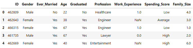
- 8068 observations in the dataset. Three numeric (Age, Work Experience and Family Size) and five categorical variables.
df.describe(include='all')

- Missing values were identified in some columns.
df.isnull().sum()
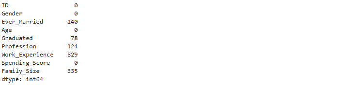
- The missing values were handled in the following way:
- Median imputation for the numeric variables.
- Adding a new standalone category named “missing” for the categorical ones.
- Then we applied FAMD by importing Prince library in Python and we used the scree plot of explained inertia to determine how many of the 8 Principal Components we would keep for our clustering.

The decision was to continue with 4 components as the bar chart becomes relatively flat from the 4th component on, whereas the first 4 PCs together explain a satisfactorily high 64% of the total inertia.
Applying FAMD for the dimension reduction
Let’s apply FAMD with 4 components to create the transformed dataset that will be used later on by the K-Means algorithm:
# Create the FAMD model with 4 components
famd = prince.FAMD(n_components=4, random_state=42)

# Fit the FAMD model on the clustering dataset and transform it
df_famd = famd.fit_transform(df_clust)
K-Means Model Implementation
How to determine the number of clusters - Elbow Method and Silhouette Score
Before running the K-Means algorithm in the new dataset df_famd, a crucial question needs to be answered: How many clusters will my observations be divided in? There are two methods to help us determine the optimal number of clusters:
- Elbow Method: This is a heuristic method which uses the plot of the WCSS (Within-Cluster Sum of Squares) — effectively the inertia — against the number of clusters. As the latter increases the former decreases since there are more clusters for each point to choose the one whose centroid it is closer to. As in the Scree Plot of the principal components, here too we are looking to stop just before we reach the number of clusters that doesn’t cause any considerable decrease in the WCSS.
- Silhouette Score: This metric shows how well defined the clusters are, by evaluating how close (or how similar) this point is to the other points in the same cluster vs how similar it is to the points of the nearest of all the other clusters. The formula for the Silhouette Score of a certain point i is given below:

Where:
ai=The average distance of the point to the points in the same cluster.
bi=The minimum of the average distances of the point to the points in each of the other clusters.
The Silhouette Score can take any value between -1 (very poor similarity to its cluster) and +1 (very strong similarity to its cluster and very poor similarity to any other cluster).
Then we calculate the average Silhouette Score of all points in the dataset.
The function below creates the plot of the WCSS for each number of clusters.
def plot_kmeans_elbow(X, k_range=range(2, 11), random_state=42):
    """Creates an elbow plot for K-Means clustering using distortion (inertia)
    in order to help select the optimal number of clusters.
    Args:
    X: array-like. The dataset used for clustering (e.g. FAMD components).
    k_range: range. Range of k values (number of clusters) to evaluate.
             Default is range(2, 11).
    random_state: int. Random seed for reproducibility of K-Means results.
    Returns:
    A line plot showing distortion (inertia) vs number of clusters.
    """
    distortions = []   # Stores K-Means inertia values for each k

    # Loop through each candidate number of clusters
    for k in k_range:
        # Create and fit K-Means model
        kmeans = KMeans(n_clusters=k, random_state=random_state)
        kmeans.fit(X)

        # Append distortion metric (sum of squared distances to centroids)
        distortions.append(kmeans.inertia_)
    # Create elbow plot
    plt.figure(figsize=(8, 5))
    plt.plot(k_range, distortions, marker='o')
    plt.xlabel("Number of clusters (k)")
    plt.ylabel("Distortion (Inertia)")
    plt.title("Elbow Method (Distortion)")
    plt.grid(True)
    plt.show()

# Apply K-Means elbow analysis on the FAMD components
plot_kmeans_elbow(df_famd)
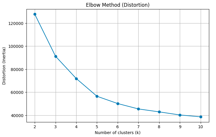
The Elbow Method suggests something between 3 and 5 clusters as the line graph is fairly straight after 5.
Let’s see the Silhouette Score (provided by the function below)
def plot_kmeans_silhouette(X, k_range=range(2, 11), random_state=42):
    """Creates a silhouette score plot for K-Means clustering
    in order to evaluate clustering quality for different k values.
    Args:
    X: array-like. The dataset used for clustering (e.g. FAMD components).
    k_range: range. Range of k values (number of clusters) to evaluate.
             Default is range(2, 11).
    random_state: int. Random seed for reproducibility of K-Means results.
    Returns:
    A line plot showing silhouette score vs number of clusters.
    """
    silhouettes = []   # Stores silhouette scores for each k

    # Loop through each candidate number of clusters
    for k in k_range:
        # Create and fit K-Means model
        kmeans = KMeans(n_clusters=k, random_state=random_state)
        labels = kmeans.fit_predict(X)   # Cluster assignments

        # Append silhouette score (mean separation quality)
        silhouettes.append(silhouette_score(X, labels))
    # Create silhouette plot
    plt.figure(figsize=(8, 5))
    plt.plot(k_range, silhouettes, marker='o')
    plt.xlabel("Number of clusters (k)")
    plt.ylabel("Silhouette Score")
    plt.title("Silhouette Analysis")
    plt.grid(True)
    plt.show()


# Apply K-Means Silhouette score analysis on the FAMD components
plot_kmeans_silhouette(df_famd)
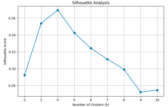
The plot confirms the finding of the previous graph as the top three scores in this plot are achieved by the number of clusters between 3 and 5. The highest score is achieved for K=4.
So the optimal number of clusters is four.
Applying K-Means algorithm
The code below shows the implementation of the K-Means algorithm with 4 clusters:
# Fit a K-Means model on the FAMD-transformed data and assign cluster labels
# The output 'labels' contains the cluster assignment for each observation
labels_km = KMeans(n_clusters=4, random_state=42).fit_predict(df_famd)

# --- K-Means clustering results applied to original data ---
# Create an independent copy of the cleaned dataset to avoid modifying the original
df_profile = df_clust.copy()

# Append the cluster labels to the dataset for profiling and analysis
df_profile.insert(0, 'Cluster', labels_km)
So our initial dataset now looks like that:
df_profile.head()

Model evaluation. 2-D and 3-D graphs of clusters
Let’s start with the Silhouette score:
# Evaluate the quality of the clustering using the silhouette score
# Higher values indicate better separation and cohesion of clusters
score = silhouette_score(df_famd, labels_km)
print('The Silhouette score for these clusters is',round(score,2))
The Silhouette score for these clusters is 0.37
As we saw in the Silhouette Analysis graph above the score is 0.37. We have also mentioned that the Silhouette Score can take any value between -1 and +1. As a general rule:
- Silhouette>0.5 -> Well separated clusters
- 0 ≤ Silhouette ≤0.5 -> Overlapping clusters
- Silhouette<0 -> Wrong clusters
So, in our case the clusters are fairly well separated (most points are well fitted within their clusters) but we should expect to see some overlap when we assess them visually below.
Next, we will summarise the clusters:
# Calculate population and population % for each of the clusters
cluster_summary = df_profile.groupby('Cluster').size().reset_index(name='Count')
cluster_summary['Percentage'] = round(cluster_summary['Count'] / cluster_summary['Count'].sum() * 100,1).astype(str)+'%'
cluster_summary
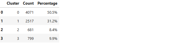
The first cluster alone contains over half the population of the dataset. The two smallest clusters are even lower than 10% of it. This doesn’t necessarily mean that the first cluster should be divided into smaller parts or that the last two should be merged with other bigger clusters. A scatter plot would give us a better insight as to how well separated the clusters are.
We will start with a 2-D scatter plot based on the first two principal components of the transformed dataset df_famd. This is what the code below achieves:
import matplotlib.patches as mpatches
# Create a new figure with a specific size
plt.figure(figsize=(10, 6))

# Extract the first two FAMD components
comp1 = df_famd.to_numpy()[:, 0]
comp2 = df_famd.to_numpy()[:, 1]

# Create a scatter plot coloured by cluster labels
scatter = plt.scatter(comp1, comp2, c=labels_km, cmap='jet')
plt.title('Cluster Visualization')   #Add title

# Label axes with explained variance -  Add grid
plt.xlabel(f'Comp 1 ({explained_inertia[0]*100:.1f}% explained)')
plt.ylabel(f'Comp 2 ({explained_inertia[1]*100:.1f}% explained)')
plt.grid(True)

# Add legend
clusters = np.unique(labels_km)   # Number of clusters
cmap = scatter.cmap   # Colourmap used by the scatter plot
norm = scatter.norm   # Normalization used by the scatter plot

# Create one legend handle per cluster:
legend_handles = [mpatches.Patch(color=cmap(norm(k)), label=f'{k}') for k in clusters]

# Draw the legend on the plot with a title and a visible frame
plt.legend(handles=legend_handles, title='Clusters', frameon=True)

plt.show()

- Remember that we had seen this scatter plot at the end of the second part (without the different colours for the clusters of course) and we had predicted two densely populated clusters at the bottom and at least one cluster at the top half.
- Clusters 0 and 1 look very compact and very well separated between them.
- There seems to be some overlap between clusters 2 and 3, even between clusters 0 and 3, which we predicted by the Silhouette Score above. But remember: This is only the first 2 of the 4 principal components that were used and the inertia they explain is 24.1%+17.2%=41.3% of the total inertia in the data.
- What about adding a third principal component? This 3-D graph should reveal a clearer relationship between these seemingly overlapping clusters.
The code below will provide it:
# Import libraries
from mpl_toolkits.mplot3d import Axes3D
from matplotlib.animation import FuncAnimation

# Create a 3D figure
fig = plt.figure(figsize=(9,9))
ax = fig.add_subplot(111, projection='3d')

# Extract the first three FAMD components
x = df_famd.to_numpy()[:, 0]
y = df_famd.to_numpy()[:, 1]
z = df_famd.to_numpy()[:, 2]

# Create a 3D scatter plot coloured by cluster labels
scatter = ax.scatter(x, y, z, c=labels_km, cmap='jet', s=40, alpha=0.8)

# Legend
clusters = np.unique(labels_km)
cmap = scatter.cmap
norm = scatter.norm
legend_handles = [mpatches.Patch(color=cmap(norm(k)),label=f'{k}') for k in clusters]
ax.legend(handles=legend_handles, title='Clusters', loc='upper right')

# Label axes with explained variance
ax.set_xlabel(f'Comp 1 ({explained_inertia[0]*100:.1f}% explained)')
ax.set_ylabel(f'Comp 2 ({explained_inertia[1]*100:.1f}% explained)')
ax.set_zlabel(f'Comp 3 ({explained_inertia[2]*100:.1f}% explained)')

ax.set_title('3D FAMD Scatter Plot')   # Add plot title

# Function to rotate the 3D view
def rotate(angle):
    ax.view_init(elev=20, azim=angle)

ani = FuncAnimation(fig, rotate, frames=range(0, 360, 2), interval=100)   # Create the rotation animation
ani.save("famd_rotation_km.gif", writer="pillow", fps=10)   # Save the animation as a GIF
plt.close(fig)   # Close the figure to prevent static display

# Display the rotating 3-D graph
from IPython.display import Image
Image(filename="famd_rotation_km.gif")

- The rotating 3-D graph shows a clearer separation between all 4 clusters although some degree of overlap is still evident.
- The first 3 components account for 24.1%+17.2%+12.2%=53.5% of the total inertia which allows for safer inference.
- Therefore having two big and two small clusters makes absolute sense, it’s the population density around the centroids that accounts for this difference.
Summary
In the third part of our series we explored these steps:
- We transformed the initial dataset by using FAMD with four Principal Components as decided in Part 2.
- We used the Elbow method for an initial estimate of the number of clusters and it returned something between three and five clusters.
- We went on with the Silhouette Score and this time we had a winner: Four clusters.
- We applied K-Means with four clusters and we evaluated the model in two ways:
- Quantitatively: Silhouette Score (effectively returned the highest score noticed in the Silhouette Scores graph presented earlier).
- Graphically: 2-D and 3-D graphs of the first two and three PCs respectively which showed a satisfactory separation between the clusters.
In the next part, we will explore an alternative ML algorithm for segmentation called Hierarchical Clustering and we will compare the results between that and K-Means as well as the pros and cons of each method.
I hope you read this article with a keen interest and enjoyed every part of it. If so, please don’t forget to give me a clap and follow me. I am also available and more than eager to connect with you on LinkedIn (Georgios Kokkinopoulos | LinkedIn).
References
[1] Cristian Leo, The Math and Code Behind K-Means Clustering | TDS Archive (2024), TDS Archive
[2] Heiko Onnen, Elbows and Silhouettes: Hands-on Customer Segmentation in Python | Towards Data Science (2021), Towards Data Science
[3] Shivam Soliya, Customer Segmentation using k-prototypes algorithm in Python | by Shivam Soliya | Analytics Vidhya | Medium (2021), Analytics Vidhya
[4] Dataset: Customer Segmentation CC0:Public Domain
[5] Github repo: GKokkinopoulos/Customer-Segmentation
Clustering Mixed Data with K-Means: From FAMD to Segments was originally published in DataDrivenInvestor on Medium, where people are continuing the conversation by highlighting and responding to this story.