In the previous post about Paged Attention, we discussed how to speed up inference by caching KV blocks. However, we are still bottlenecked by the number of serial forward passes. Today, we’re going to continue along that line of thinking and introduce speculative decoding to NanoGPT.
Problem
In real world inference systems, standard auto-regressive decoding is sequential. Each token requires one full forward pass of the model. Even with the KV cache, you are bottlenecked by the number of serial forward passes.
Step 1: forward(token_0) → token_1
Step 2: forward(token_1) → token_2
Step 3: forward(token_2) → token_3
...
N tokens = N forward passes
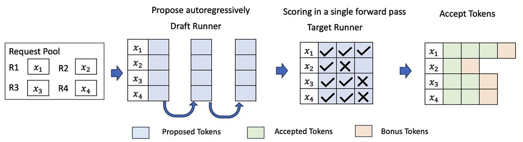
Speculative decoding breaks this by using a cheap draft model to guess K tokens ahead, then verifying all K guesses in a single forward pass of the real (target) model. If the guesses are good, you get K+1 tokens for the cost of ~1 target forward pass.
Draft:  guess token_1, token_2, token_3, token_4  (cheap, ~free)
Verify: forward([token_0, token_1, token_2, token_3, token_4]) → check all at once
Accept: token_1 ✓, token_2 ✓, token_3 ✗ → resample token_3 from target
Result: 3 tokens from 1 target forward pass!
It guarantees that the output distribution is mathematically identical to the target model alone. Speculative decoding never degrades quality — it only speeds things up (or, in the worst case, matches normal decoding speed).
The Algorithm at a Glance
┌─────────────────────────────────────────────────────────────────┐
│                   SPECULATIVE DECODING LOOP                     │
│                                                                 │
│   ┌──────────┐     ┌──────────┐     ┌────────────┐     ┌─────┐ │
│   │  DRAFT   │────▶│  VERIFY  │────▶│   ACCEPT   │────▶│TRIM │ │
│   │          │     │          │     │  / REJECT   │     │ KV  │ │
│   │ Bigram   │     │ 1 target │     │             │     │CACHE│ │
│   │ guesses  │     │ forward  │     │ Rejection   │     │     │ │
│   │ K tokens │     │ pass for │     │ sampling on │     │Keep │ │
│   │ (cheap!) │     │ all K at │     │ each draft  │     │only │ │
│   │          │     │ once     │     │ token       │     │valid│ │
│   └──────────┘     └──────────┘     └────────────┘     └──┬──┘ │
│        ▲                                                   │    │
│        └───────────────────────────────────────────────────┘    │
│                        repeat until done                        │
└─────────────────────────────────────────────────────────────────┘
A Worked Example
Let’s make this concrete. Say the target model has generated "To be or not to be, that is the " and current_token = "t". We speculate with K=4:
DRAFT (bigram model guesses 4 tokens):
  "t" → "h" → "e" → " " → "q"
  candidates = ["h", "e", " ", "q"]

VERIFY (target model scores all 4 in one forward pass):
  target sees: ["t", "h", "e", " ", "q"]
  target_probs[0] → P(next | ..."the ") for checking "h"  ← high prob ✓
  target_probs[1] → P(next | ..."the h") for checking "e" ← high prob ✓
  target_probs[2] → P(next | ..."the he") for checking " " ← hmm, low prob
  target_probs[3] → P(next | ..."the he ") for checking "q"
ACCEPT/REJECT (check each candidate left-to-right):
  "h" → p/q = 0.92/0.31 = 2.97 → min(1, 2.97) = 1.0  → ✅ ACCEPT
  "e" → p/q = 0.88/0.40 = 2.20 → min(1, 2.20) = 1.0  → ✅ ACCEPT
  " " → p/q = 0.05/0.35 = 0.14 → rand(0.71) > 0.14   → ❌ REJECT
        resample from adjusted distribution → "a" (for "heap")
        STOP - discard remaining candidates
RESULT: accepted = ["h", "e", "a"]
         3 tokens from 1 target forward pass (instead of 3 forward passes)
TRIM KV CACHE:
  Cache had entries for ["t", "h", "e", " ", "q"] from verification
  Keep only ["t", "h", "e"], discard [" ", "q"]
  "a" becomes the new current_token for the next round
Even with a simple bigram draft model that gets rejected fairly often, we still generated 3 tokens from a single expensive forward pass. On longer sequences with a better draft model, acceptance rates climb and the speedups become dramatic.
Here is what we have so far:
• ✅ GPTLanguageModel with stateless Head.forward() and KV cache support
• ✅ model.forward(idx, pos=pos, past_kvs=past_kvs) returns (logits, loss, new_kvs)
• ✅ The model can process multiple tokens at once: idx shape (B, T) where T > 1
• ✅ Training data (input.txt — Tiny Shakespeare) for building a bigram table
• ✅ encode() / decode() for tokenization
It is important to note that at our scale (210k parameters), trying to do speculative decoding doesn’t make much sense from a performance perspective. But it is important for learning purposes to show that this possible. We will be using a bigram table to generate our draft tokens.
Bigram Table
class BigramDraftModel:
    """
    Draft model for speculative decoding.
    Predicts P(next_token | current_token) from training data statistics.
    """
    def __init__(self, train_data, vocab_size, device):
        # Count bigram frequencies: how often does token B follow token A?
        counts = torch.zeros(vocab_size, vocab_size, device=device)
        for i in range(len(train_data) - 1):
            counts[train_data[i], train_data[i + 1]] += 1

    # Convert counts to probabilities (add smoothing to avoid zeros)
        counts += 1  # Laplace smoothing
        self.probs = counts / counts.sum(dim=1, keepdim=True)  # (vocab_size, vocab_size)
    def get_probs(self, token_id):
        """Return P(next | token_id) as a (vocab_size,) distribution."""
        return self.probs[token_id]
    def sample(self, token_id):
        """Sample one token given the current token."""
        probs = self.get_probs(token_id)
        return torch.multinomial(probs, num_samples=1).item(), probs
Build the count matrix. The constructor takes the entire training corpus (train_data) and scans it once from left to right. For every consecutive pair of tokens (A, B), it increments counts[A, B] by 1. The result is a (vocab_size, vocab_size) matrix where row A records how many times each token B appeared immediately after token A in the training data. For Tiny Shakespeare with a character-level tokenizer (~65 unique characters), this is a tiny 65×65 matrix — it fits trivially in GPU memory.
Apply Laplace smoothing. Before normalizing, we add 1 to every cell (counts += 1). Without this, any bigram that never appeared in the training data would have probability 0, which causes two problems: (1) torch.multinomial crashes if the entire distribution is zero, and (2) during the speculative decoding acceptance step, dividing by a draft probability of 0 would produce infinity. Laplace smoothing ensures every transition has at least a tiny non-zero probability. The trade-off is that the distribution is slightly less sharp — but for a draft model that only needs to be "roughly right" most of the time, this is perfectly acceptable.
Normalize to probabilities. counts / counts.sum(dim=1, keepdim=True) divides each row by its total, converting raw counts into a proper probability distribution where each row sums to 1. After this, self.probs[A] is a valid categorical distribution over all possible next tokens given that the current token is A.
get_probs(token_id). A simple row lookup — returns the full (vocab_size,) probability distribution for the next token given token_id. This is an O(1) table lookup, which is why the bigram model is essentially "free" compared to a transformer forward pass.
sample(token_id). Draws one token from the bigram distribution using torch.multinomial, which samples from the categorical distribution weighted by the probabilities. Critically, this method returns both the sampled token ID and the full probability distribution probs. The reason we return the distribution is that the speculative decoding acceptance step needs it later — to decide whether to accept or reject a draft token, the algorithm compares P_target(token) / P_draft(token), so we need to know what probability the draft model assigned to each guess.
The bigram table in our case is basically a free lookup since we aren’t doing a full separate transformer pass. The bigram table cannot capture long range dependencies, but even with a 30% acceptance rate, we can still sometimes get 2–3 tokens per target forward pass instead of one.
The Draft Phase — Generating K Candidates
The draft phase is simple: autoregressively sample K tokens from the bigram model, storing the draft probabilities for each.
Draft Phase (Sequential Generation):
[current_token] ──▶ Draft Model ──▶ c0
                                    │
                                    ▼
                                   [c0] ──▶ Draft Model ──▶ c1
                                                            │
                                                            ▼
                                                           [c1] ──▶ Draft Model ──▶ c2
def draft_tokens(draft_model, current_token, K):
    """
    Generate K speculative tokens from the draft model.
    Returns:
        candidates:  list of K token ids
        draft_probs: list of K probability distributions (each is (vocab_size,))
    """
    candidates = []
    draft_probs = []
    tok = current_token
    for _ in range(K):
        next_tok, probs = draft_model.sample(tok)
        candidates.append(next_tok)
        draft_probs.append(probs)
        tok = next_tok
    return candidates, draft_probs
In the draft phase, we simply call draft_model.sample() K times in a loop. Each call returns a single token and its probability distribution. We collect these into candidates (the sequence of token IDs) and draft_probs (the sequence of distributions). This is done entirely with the draft model, so it's very fast — for our bigram model, it's just table lookups and random sampling, no matrix multiplications.
The Verification Phase — One Target Forward Pass
This is the key insight: the target model can verify all K candidates in a single forward pass because of the causal attention structure.
Verification Phase (Parallel Scoring):
       [current_token]        [c0]             [c1]             [c2]
              │                │                │                │
              ▼                ▼                ▼                ▼
    ┌──────────────────────────────────────────────────────────────────┐
    │                    Target Model (1 Forward Pass)                 │
    └──────────────────────────────────────────────────────────────────┘
              │                │                │                │
              ▼                ▼                ▼                ▼
        target_probs[0]  target_probs[1]  target_probs[2]  target_probs[3]
        (scores c0)      (scores c1)      (scores c2)      (scores bonus)
You feed the target model the sequence [current_token, candidate_0, candidate_1, ..., candidate_{K-1}] as a (1, K+1) input. The model produces logits at every position. The logit at position i gives the target model's distribution for what should come after position i.
def verify_candidates(target_model, current_token, candidates, past_kvs):
    """
    Run the target model on [current_token] + candidates in one forwacrd pass.
    Returns:
        target_probs: list of K+1 probability distributions
        new_kvs:      updated KV cache
    """
    # Build input: [current_token, c0, c1, ..., c_{K-1}]
    all_tokens = [current_token] + candidates
    input_ids = torch.tensor([all_tokens], dtype=torch.long, device=device)
    # Position indices continue from where the cache left off
    cache_len = 0  # number of tokens already in the KV cache
    if past_kvs is not None:
        # Get T_past from the first layer, first head's key tensor
        cache_len = past_kvs[0][0][0].shape[1]
    positions = torch.arange(cache_len, cache_len + len(all_tokens), device=device).unsqueeze(0)
    # Single forward pass!
    logits, _, new_kvs = target_model(input_ids, pos=positions, past_kvs=past_kvs)
    # logits shape: (1, K+1, vocab_size)
    # Convert to probabilities
    target_probs = []
    for i in range(len(all_tokens)):
        probs = F.softmax(logits[0, i, :], dim=-1)
        target_probs.append(probs)
    return target_probs, new_kvs
Assemble the input sequence. all_tokens = [current_token] + candidates builds a single sequence of K+1 tokens: the last accepted token followed by the K draft guesses. This gets wrapped in a (1, K+1) tensor — batch size 1, sequence length K+1. The key insight is that thanks to causal attention, the model can process all K+1 tokens in parallel: position i can only attend to positions 0..i, so each position's output is computed as if the draft tokens before it were the real sequence. This is why verification costs one forward pass regardless of K.
Continue positions from the KV cache. If we’ve already generated tokens in previous steps, those KV tensors are stored in past_kvs. We read the cache length from past_kvs[0][0][0].shape[1] (the sequence dimension of the first layer's first head's key tensor) to know where to start numbering positions. For example, if 10 tokens are already cached and we're verifying 5 candidates, positions will be [10, 11, 12, 13, 14]. Getting this wrong would produce incorrect positional embeddings and garbled attention — a subtle bug that silently degrades output quality without crashing.
Single forward pass. target_model(input_ids, pos=positions, past_kvs=past_kvs) runs the full transformer on all K+1 tokens at once. The output logits has shape (1, K+1, vocab_size). Position 0's logits represent the target model's opinion on what should follow current_token — this is what we'll compare against the draft's first guess. Position 1's logits represent what should follow candidate_0 given the full context [..., current_token, candidate_0], and so on. The updated new_kvs contains KV entries for all K+1 new positions, which we'll need to trim later based on how many candidates are accepted.
Convert logits to probabilities. We loop through each position and apply F.softmax to convert raw logits into a proper probability distribution. We get K+1 distributions: target_probs[0] is the target's distribution for verifying candidate_0, target_probs[1] for verifying candidate_1, and so on. The extra target_probs[K] (the last one) is the target model's distribution for the token after the last candidate — this is used as a "bonus" token if all K candidates are accepted.
Return both probs and the updated cache. The caller (the accept/reject step) needs target_probs to compare against draft_probs for each candidate. It also needs new_kvs — but with a caveat: if some candidates are rejected, the KV cache entries for the rejected positions must be rolled back. We'll handle that trimming in the main speculative decoding loop.
Visualizing positions Allocation
Imagine we have already processed and verified 6 tokens (which are now stored in our target model’s KV cache). cache_len = 6 (occupying absolute sequence indices 0 to 5).
We are running a speculation step with K = 3 candidates: [c0, c1, c2]. all_tokens = [current_token, c0, c1, c2] (length = 4).
Here is how the absolute positional indices are mapped out visually:
Sequence Timeline:
[   Previously Verified (In KV Cache)   ] [ Current ] [           Speculative Candidates           ]
[  t0  ,  t1  ,  t2  ,  t3  ,  t4  ,  t5  ] [cur_tok] [    c0     ,       c1       ,       c2       ]

Absolute Logical Positions:
   0      1      2      3      4      5       6             7               8               9
                                              ▲             ▲               ▲               ▲
                                          cache_len    cache_len+1     cache_len+2     cache_len+3
                                              │             │               │               │
                                              └─────────────┴───────┬───────┴───────────────┘
                                                                    │
                                                 positions = torch.arange(6, 6 + 4)
                                                 positions = [6, 7, 8, 9]
• Why this offset is necessary: The positional embedding matrix expects absolute position indices to add spatial information. By querying positions [cache_len, …, cache_len + K], the transformer computes the correct positional embeddings for the brand-new incoming tokens relative to the pre-existing cached sequence context.
Why does this work? Position i in the output only attends to positions ≤ i (causal masking). So:
• target_probs[0] = P(next | prompt, current_token) — what the target thinks should follow current_token
• target_probs[1] = P(next | prompt, current_token, c0) — what should follow c0
• target_probs[i] = P(next | prompt, current_token, c0, …, c_{i-1}) — what should follow c_{i-1}
This lets you check each candidate against what the target model actually wanted.
The Accept/Reject Phase — Rejection Sampling
This is the mathematically precise part. For each draft token, you decide whether to accept it based on how well the draft model’s prediction matches the target model’s prediction.
Acceptance Math (p = target_prob, q = draft_prob):

Scenario A: Target likes token MORE than Draft did (p > q)
  p = 0.8, q = 0.4  ──▶  p/q = 2.0  ──▶  min(1, 2.0) = 1.0  ──▶  100% Accept
Scenario B: Target likes token LESS than Draft did (p < q)
  p = 0.2, q = 0.8  ──▶  p/q = 0.25 ──▶  min(1, 0.25) = 0.25 ──▶  25% Accept, 75% Reject
def accept_reject(candidates, draft_probs, target_probs):
    """
    Apply rejection sampling to decide which draft tokens to accept.

    Args:
        candidates:   list of K draft token ids
        draft_probs:  list of K draft probability distributions
        target_probs: list of K+1 target probability distributions
                      (target_probs[i] is the target's distribution for position i)
    Returns:
        accepted_tokens: list of accepted tokens (1 to K+1 tokens)
    """
    accepted = []
    for i in range(len(candidates)):
        token = candidates[i]
        q = draft_probs[i][token]    # draft model's probability for this token
        p = target_probs[i][token]   # target model's probability for this token
        # Accept with probability min(1, p/q)
        if torch.rand(1, device=p.device).item() < (p / q).clamp(max=1.0).item():
            accepted.append(token)
        else:
            # Rejected! Resample from the adjusted distribution
            # The adjusted distribution ensures we match the target exactly
            adjusted = torch.clamp(target_probs[i] - draft_probs[i], min=0)
            adjusted = adjusted / adjusted.sum()
            resampled = torch.multinomial(adjusted, num_samples=1).item()
            accepted.append(resampled)
            return accepted  # Stop here - don't check further candidates
    # All K candidates accepted! Sample one bonus token from the target
    bonus = torch.multinomial(target_probs[len(candidates)], num_samples=1).item()
    accepted.append(bonus)
    return accepted
Loop through candidates left-to-right. We check each draft token sequentially, starting from candidate_0. Order matters — if candidate_2 is rejected, we can't trust anything after it because those later candidates were drafted conditioned on candidate_2 being correct. This is why rejection at position i immediately stops the loop and discards all subsequent candidates.
Look up both probabilities for the draft token. For each candidate token, we read two numbers: q = draft_probs[i][token] (the probability the draft model assigned to this token) and p = target_probs[i][token] (the probability the target model assigned to the same token). If the draft model was perfect (p == q everywhere), every token would be accepted. If the draft model is bad (high q for tokens the target assigns low p), most tokens get rejected.
Accept with probability min(1, p/q). This is the core of rejection sampling. We draw a uniform random number and accept if it's less than p/q (clamped to 1). The intuition: if the target model thinks the token is more likely than the draft did (p > q), we always accept (probability = 1). If the target thinks it's less likely (p < q), we accept proportionally — e.g., if p/q = 0.3, we accept 30% of the time. This guarantees that accepted tokens follow the target distribution exactly, not the draft distribution. This is the mathematical property that makes speculative decoding lossless — it never degrades output quality.
On rejection: resample from the adjusted distribution. When a candidate is rejected, we don’t just discard it — we need to produce a valid token for this position. The adjusted distribution max(0, p - q) (normalized) represents the "residual" probability mass that the target model assigns but the draft model under-represents. Sampling from this distribution, combined with the acceptance step above, is mathematically proven to produce the exact same token distribution as sampling directly from the target model. Without this correction, rejection would introduce bias — you'd be systematically under-representing tokens that the draft model favors.
Early return on rejection. return accepted immediately exits the function after appending the resampled token. All subsequent candidates (candidate_{i+1}, ..., candidate_{K-1}) are thrown away because they were drafted assuming the rejected token was correct — their draft probabilities are conditioned on a wrong prefix. In the worst case (first token rejected), we get exactly 1 token from this step — the same as normal autoregressive decoding. Speculative decoding never does worse than standard decoding.
Bonus token on full acceptance. If all K candidates pass, we’ve gotten K tokens essentially for free. But we also have target_probs[K] — the target model's distribution for the position after the last candidate — sitting there from the verification forward pass. We sample one more token from it for free, yielding K+1 total tokens from a single target forward pass. This is the best-case scenario and the source of speculative decoding's speedup.
KV Cache Management
The tricky part: after accept/reject, you need to trim the KV cache to match only the accepted tokens. The verification forward pass cached KV entries for all K+1 tokens, but if you only accepted 2 of them, the cache entries for positions 3, 4, 5 are invalid.
def trim_kv_cache(new_kvs, num_accepted, cache_len_before_verify):
    """
    Trim the KV cache to only include accepted tokens.
    After verification, the cache has entries for all K+1 speculative tokens.
    We need to keep only the first `num_accepted` new entries.
    Args:
        new_kvs:     KV cache from the verification forward pass
        num_accepted: how many tokens were accepted
        cache_len_before_verify: KV cache length before the verify call
    """
    keep = cache_len_before_verify + num_accepted
    trimmed = []
    for layer_kv in new_kvs:
        layer_trimmed = []
        for (k, v) in layer_kv:
            layer_trimmed.append((k[:, :keep, :], v[:, :keep, :]))
        trimmed.append(layer_trimmed)
    return trimmed
Why trim? If you accepted tokens [A, B] but rejected C (and resampled C'), your KV cache from the verify pass contains entries computed assuming the sequence was [..., A, B, C]. But the actual sequence is [..., A, B, C']. The KV entries for C are wrong — they were computed with the wrong token. You must discard them.
Visualizing trim_kv_cache
Assume K = 3 candidates drafted: [c0, c1, c2] Input to verify: [cur_tok, c0, c1, c2] The verification step produces new_kvs which contains KV entries for all 4 of these tokens.
Scenario: c0 is accepted, but c1 is rejected. The accept/reject logic replaces c1 with resampled_c1 and stops. It returns: accepted = [c0, resampled_c1] (length = 2).
Here is how the KV cache is trimmed:
KV Cache before trimming (from verification step):
[ ...past_kvs... ] [ cur_tok ] [   c0   ] [   c1   ] [   c2   ]
                   └────────────────── new_kvs ─────────────────┘

Trimming operation (keep = cache_len + 2):
[ ...past_kvs... ] [ cur_tok ] [   c0   ] ✂️ discarded (c1, c2) ✂️
Resulting KV Cache:
[ ...past_kvs... ] [ cur_tok ] [   c0   ]
Current Generated Sequence:
[ ...prompt...   ] [ cur_tok ] [   c0   ] [ resampled_c1 ]
Notice the perfect alignment: the KV cache contains everything up to c0. The very last token in our sequence, resampled_c1, is not in the KV cache yet. This perfectly maintains our invariant! In the next speculation step, resampled_c1 will be passed in as the new cur_tok, and its KV entry will be computed then
Putting it Together
@torch.no_grad()
def speculative_generate(target_model, draft_model, prompt_tokens, max_new_tokens, K=4):
    target_model.eval()
    generated = []

# 1. Prefill: run the full prompt through the target model
    input_ids = torch.tensor([prompt_tokens], dtype=torch.long, device=device)
    positions = torch.arange(len(prompt_tokens), device=device).unsqueeze(0)
    logits, _, past_kvs = target_model(input_ids, pos=positions)
    # Sample the first token from the prefill output
    probs = F.softmax(logits[0, -1, :], dim=-1)
    current_token = torch.multinomial(probs, num_samples=1).item()
    generated.append(current_token)
    # 2. Speculative decode loop
    while len(generated) < max_new_tokens:
        cache_len = past_kvs[0][0][0].shape[1]  # current KV cache length
        # How many tokens to speculate (don't overshoot max_new_tokens)
        k = min(K, max_new_tokens - len(generated))
        # DRAFT
        candidates, draft_probs = draft_tokens(draft_model, current_token, k)
        # VERIFY
        target_probs, new_kvs = verify_candidates(
            target_model, current_token, candidates, past_kvs
        )
        # ACCEPT/REJECT
        accepted = accept_reject(candidates, draft_probs, target_probs)
        # TRIM KV CACHE (keep only accepted tokens)
        past_kvs = trim_kv_cache(new_kvs, len(accepted), cache_len)
        # Update state
        generated.extend(accepted)
        current_token = accepted[-1]
    return generated[:max_new_tokens]
Prefill the prompt. Before any speculation can happen, we need the target model to process the full prompt and build its KV cache. We feed all prompt_tokens as a (1, T) tensor with positions [0, 1, ..., T-1]. The model returns logits for every position, but we only care about the last one — logits[0, -1, :] — which gives us the target model's distribution for the first generated token. We sample from it, append to generated, and now have a primed KV cache (past_kvs) containing all the prompt's key-value pairs ready for the speculation loop.
The four-step speculative loop. Each iteration runs the full draft → verify → accept/reject → trim cycle. The while loop continues until we’ve generated max_new_tokens tokens, with each iteration potentially producing anywhere from 1 token (worst case: first draft token rejected) to K+1 tokens (best case: all drafts accepted plus a bonus token).
Clamp k to avoid overshooting. k = min(K, max_new_tokens - len(generated)) ensures we don't speculate more tokens than we actually need. Without this, the last iteration might generate 5 tokens when we only needed 2 more, and the final generated[:max_new_tokens] slice would silently discard work. This is a minor optimization — the slice at the end is the safety net — but it avoids wasting forward pass compute on tokens we'll throw away.
Draft, verify, accept/reject, trim. These four lines are just calls to the functions we’ve already built. The order is critical: draft_tokens proposes K guesses cheaply, verify_candidates scores them all in one target forward pass, accept_reject decides which to keep using rejection sampling, and trim_kv_cache rolls back the KV cache to match the accepted prefix. Each function is stateless and composable — all shared state flows through past_kvs and current_token.
Update state for the next iteration. We append all accepted tokens to generated and set current_token to the last accepted token. This maintains the invariant that current_token is always the most recent token not yet in the KV cache. In the next iteration, it will be passed into both draft_tokens (as the seed for bigram sampling) and verify_candidates (as the first element of the verification input). The KV cache at this point contains everything up to but not including current_token — exactly what the next verification pass needs.
Conclusion
Speculative decoding is one of those rare optimization techniques that feels like magic: it guarantees the exact same output quality as standard autoregressive generation, but can significantly reduce the wall-clock time required to generate it. By breaking the serial bottleneck of the LLM forward pass, we effectively trade cheap, abundant compute (parallel verification) for a reduction in expensive, latency-bound compute (sequential token generation).
While our simple bigram draft model on a 210k parameter NanoGPT is more of an educational toy, the core principles we just implemented are identical to what runs in production. Modern inference engines like vLLM and TensorRT-LLM rely heavily on speculative decoding — usually using smaller, specialized transformer models as drafters — to serve massive models efficiently at scale.
If you want to see the complete implementation, including the greedy equivalence tests that prove the math works perfectly, you can find the rest of the code here: https://github.com/czhou578/multimodal-inference-visualizer/blob/main/nanogpt-speculative-decoding.ipynb
Colin Zhou
Adding Speculative Decoding to Andrej Karpathy’s NanoGPT (2026 edition) was originally published in Level Up Coding on Medium, where people are continuing the conversation by highlighting and responding to this story.