Activation Functions in JAX: A Deep Dive into Neural Network Non-Linearities

If you have ever trained a deep neural network that refused to learn, produced exploding loss values, or mysteriously plateaued long before reaching reasonable accuracy, there is a very good chance the culprit was your activation function. This tutorial takes a deep dive at six popular activation functions: Sigmoid, Tanh, ReLU, LeakyReLU, ELU, and Swish implementing each from scratch in JAX. By the end, you will have a clear mental model for choosing the right activation function.

Why Activation Functions Matter

Before diving into code, it is worth spending a moment on the “why.” A neural network without activation functions is mathematically just a linear transformation of its input, no matter how many layers you stack. The composition of linear functions is still linear, which means that a ten-layer network with no non-linearity is strictly equivalent to a single weight matrix, hardly the kind of universal function approximator we want.

Activation functions introduce non-linearity at each layer, allowing the network to model highly complex relationships in data. But not all non-linearities are created equal. Some introduce training hurdles:

Vanishing gradients: When the gradient of the activation function is consistently much smaller than 1 across large portions of the input space, the signal that propagates back through many layers becomes exponentially small, and early layers learn nothing.
Exploding gradients: The mirror image problem when gradients grow exponentially as they travel backward, destabilizing training.
Dead neurons: A neuron whose output is permanently zero for all inputs in the training set. It contributes nothing to the forward pass, and because its gradient is zero it can never recover via back-propagation.

Choosing a good activation function means navigating all three failure modes simultaneously, while also considering computational cost, the smoothness properties that some optimizers expect, and how the function interacts with weight initialization schemes. This tutorial walks through each of these considerations methodically, using JAX to make the analysis concrete and reproducible.

Implementing and Visualizing Six Activation Functions

We are going to implement each activation function as a plain JAX function using jax.numpy operations. This means each one automatically becomes differentiable via jax.grad, JIT-compilable via jax.jit, and vectorizable via jax.vmap. We get all of that for free just by writing functions in terms of jnp operations.

We will also write a helper that plots both the activation function itself and its derivative side by side, so we can immediately see the gradient landscape.


import os
import math
import time
from functools import partial
from typing import Callable, Sequence, Any
# Scientific stack 
import numpy as np
import matplotlib.pyplot as plt
import matplotlib.colors as colors
from matplotlib import cm
# JAX + Flax + Optax 
import jax
import jax.numpy as jnp
from jax import random, grad, jit, vmap


def plot_activation(fn: Callable, fn_name: str, x_range: tuple = (-5, 5)):
    """Plot an activation function and its gradient."""
    x = jnp.linspace(x_range[0], x_range[1], 1000)
    y = fn(x)
    # Use vmap(grad(fn)) to compute element-wise gradient
    dy = vmap(grad(fn))(x)
    fig, axes = plt.subplots(1, 2, figsize=(10, 3.5))
    fig.suptitle(f"Activation: {fn_name}", fontsize=14, fontweight="bold")
    axes[0].plot(x, y, color="steelblue", linewidth=2)
    axes[0].axhline(0, color="black", linewidth=0.6, linestyle="--")
    axes[0].axvline(0, color="black", linewidth=0.6, linestyle="--")
    axes[0].set_xlabel("Input x")
    axes[0].set_ylabel("f(x)")
    axes[0].set_title("Activation function")
    axes[0].grid(True, alpha=0.3)
    axes[1].plot(x, dy, color="darkorange", linewidth=2)
    axes[1].axhline(0, color="black", linewidth=0.6, linestyle="--")
    axes[1].axvline(0, color="black", linewidth=0.6, linestyle="--")
    axes[1].set_xlabel("Input x")
    axes[1].set_ylabel("f'(x)")
    axes[1].set_title("Gradient (derivative)")
    axes[1].grid(True, alpha=0.3)
    plt.tight_layout()
    plt.show()

Sigmoid Function

The sigmoid function maps any real number to the open interval (0, 1):

σ(x) = 1 / (1 + exp(-x))

It was the go-to activation function in the early days of neural networks because its output can be interpreted as a probability. However, it has a well-known flaw: its gradient is at most 0.25, reached at x = 0, and decays rapidly toward zero as |x| grows. In a deep network, multiplying many such small gradients together as we propagate backward means the signal reaching early layers can be become very small, the classic vanishing gradient problem.

def sigmoid(x: jnp.ndarray) -> jnp.ndarray:
    """
    Sigmoid activation function.
    σ(x) = 1 / (1 + exp(-x))
    Output range: (0, 1)
    Max gradient: 0.25 at x=0
    """
    return 1.0 / (1.0 + jnp.exp(-x))

plot_activation(sigmoid, "Sigmoid")

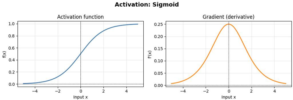
Key properties:

Output is strictly in (0, 1), making it natural for binary classification output layers.
Gradient is symmetric around x = 0 and reaches a maximum of exactly 0.25.
For |x| > 4, the gradient is effectively zero , the function is saturated, and no learning signal flows through it.
Outputs are not zero-centered, which can slow down convergence in the first layer.

Tanh Function

The hyperbolic tangent is closely related to sigmoid, but it is zero-centered, mapping to (−1, 1):

tanh(x) = (exp(x) − exp(−x)) / (exp(x) + exp(−x))

def tanh(x: jnp.ndarray) -> jnp.ndarray:
    """
    Hyperbolic tangent activation.
    tanh(x) = (exp(x) - exp(-x)) / (exp(x) + exp(-x))
    Output range: (-1, 1)
    Max gradient: 1.0 at x=0
    """
    return jnp.tanh(x)  # JAX has a numerically stable built-in

plot_activation(tanh, "Tanh")

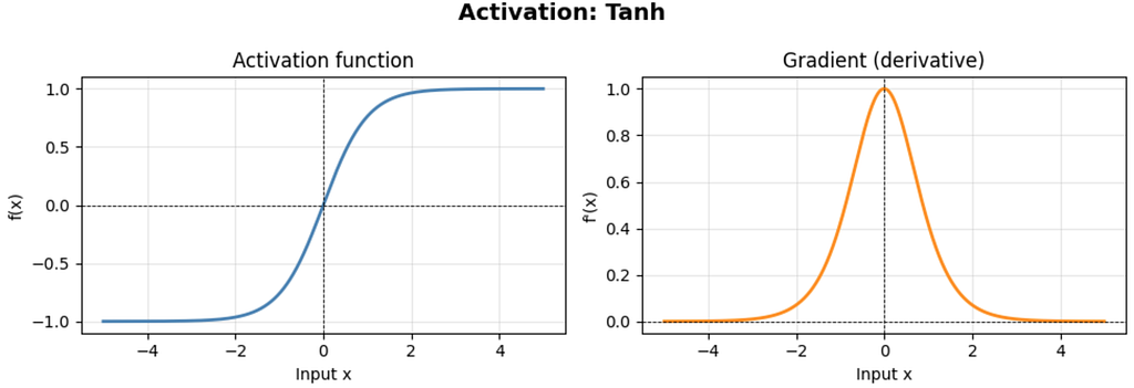
Key properties:

Zero-centered output, which is generally preferable to sigmoid for hidden layers.
Maximum gradient of 1.0 at x = 0, four times larger than sigmoid’s maximum.
Still suffers from saturation for |x| > 2 and therefore still causes vanishing gradients in very deep networks.
The gradient can reach 1.0, which is better than sigmoid, but does not guarantee gradient flow. For large pre-activation values the gradient still collapses.

Both sigmoid and tanh were dominant for decades before the community rediscovered and embraced ReLU, whose gradient properties are dramatically better for deep networks.

ReLU Function

The Rectified Linear Unit is a simple function:

ReLU(x) = max(0, x)

Its gradient is 1 for positive inputs and 0 for negative inputs. This property helps preserve the gradients flowing through ReLU neurons with positive pre-activations. This is why very deep networks (10, 20, even 100+ layers) became practically trainable once ReLU replaced sigmoid and tanh in hidden layers.

def relu(x: jnp.ndarray) -> jnp.ndarray:
    """
    Rectified Linear Unit.
    ReLU(x) = max(0, x)
    Output range: [0, ∞)
    Gradient: 1 for x > 0, 0 for x < 0
    """
    return jnp.maximum(0, x)

plot_activation(relu, "ReLU")

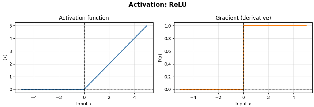
Key properties:

Gradient of exactly 1 for all positive inputs, no vanishing gradient for active neurons.
Computationally trivial: just a comparison and a clip.
Output is not zero-centered, which can cause some optimization inefficiency.
The dying ReLU problem: if the pre-activation of a neuron is negative for every training example, its gradient is always 0 and its upstream weights receive no updates. The neuron is permanently dead and wastes capacity.

The dying ReLU problem is prominent when learning rates are high or weight initialization is poor, causing large fractions of neurons to fire negatively and never recover. All three activation functions that follow attempt to address this, each in a slightly different way.

LeakyReLU Function

The most straightforward fix: instead of setting the output to zero for negative inputs, allow a small positive gradient through:

LeakyReLU(x) = x         if x ≥ 0
             = α·x        if x < 0

where α is a small constant, typically 0.01.

def leaky_relu(x: jnp.ndarray, alpha: float = 0.01) -> jnp.ndarray:
    """
    Leaky ReLU.
    f(x) = x for x >= 0, alpha * x for x < 0
    Output range: (-∞, ∞)
    Gradient: 1 for x > 0, alpha for x < 0
    """
    return jnp.where(x >= 0, x, alpha * x)
plot_activation(leaky_relu, "LeakyReLU")

Key properties:

Gradient of α (e.g. 0.01) for negative inputs and neurons can never die completely.
Essentially identical to ReLU for positive inputs.
In practice the improvement over plain ReLU is modest and inconsistent; the α hyper-parameter is another thing to tune.
The parametric variant, PReLU, makes α a learnable parameter per channel, which sometimes works better.

ELU Function

The Exponential Linear Unit replaces the hard zero floor for negative inputs with a smooth exponential curve that asymptoticly converges to −α:

ELU(x) = x              if x > 0
       = α·(exp(x) − 1) if x ≤ 0

where α is typically 1.0.

def elu(x: jnp.ndarray, alpha: float = 1.0) -> jnp.ndarray:
    """
    Exponential Linear Unit.
    f(x) = x for x > 0, alpha * (exp(x) - 1) for x <= 0
    Output range: (-alpha, ∞)
    Saturates to -alpha for very negative inputs.
    """
    return jnp.where(x > 0, x, alpha * (jnp.exp(x) - 1.0))
plot_activation(elu, "ELU")

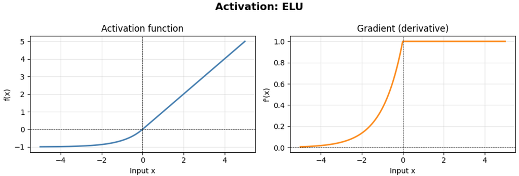
Key properties:

Smooth everywhere (unlike ReLU and LeakyReLU which have a kink at 0).
The negative part saturates to −α instead of being linear, which provides a form of noise robustness . High negative valued corrupted inputs still produce a bounded, informative output.
Mean activation is closer to zero than ReLU, which helps with internal covariant shift.
More expensive to compute than ReLU or LeakyReLU because of the exp call on the negative half.

Swish Function

Swish emerged from a large-scale automated search for better activation functions conducted by Google Brain researchers.

Swish(x) = x · σ(x) = x / (1 + exp(-x))

This is also known as SiLU (Sigmoid Linear Unit). What makes Swish distinctive is that it is both smooth and non-monotonic, unlike all the functions we have seen so far, it has a small dip near x ≈ −1.3 where the output is slightly negative before recovering. This non-monotonicity has been empirically shown to be beneficial for very deep networks.

def swish(x: jnp.ndarray) -> jnp.ndarray:
    """
    Swish (SiLU) activation function.
    f(x) = x * sigmoid(x) = x / (1 + exp(-x))
    Output range: (-∞, ∞), non-monotonic
    Smooth and differentiable everywhere.
    """
    return x * sigmoid(x)
plot_activation(swish, "Swish")

Key properties:

Smooth everywhere, unbounded above, and softly bounded below (does not hard-saturate).
Non-monotonic: the small negative dip means the gradient can change sign, which provides richer gradient information.
Performs comparably to or better than ReLU on very deep networks and has become the default in many modern architectures (Mish, another variant, extends the idea further).
Slightly more expensive than ReLU due to the sigmoid computation.

Comparing All Six at Once

activation_fns = {
    "Sigmoid": sigmoid,
    "Tanh": tanh,
    "ReLU": relu,
    "LeakyReLU": leaky_relu,
    "ELU": elu,
    "Swish": swish,
}

fig, axes = plt.subplots(2, 3, figsize=(15, 8))
x = jnp.linspace(-5, 5, 1000)
for ax, (name, fn) in zip(axes.flatten(), activation_fns.items()):
    y = fn(x)
    dy = vmap(grad(fn))(x)
    ax.plot(x, y, label="f(x)", color="steelblue", linewidth=2)
    ax.plot(x, dy, label="f'(x)", color="darkorange", linewidth=2, linestyle="--")
    ax.axhline(0, color="black", linewidth=0.5)
    ax.axvline(0, color="black", linewidth=0.5)
    ax.set_title(name, fontsize=12, fontweight="bold")
    ax.legend()
    ax.grid(True, alpha=0.3)
    ax.set_ylim(-2, 3)
plt.suptitle("Activation Functions and Their Gradients", fontsize=14, fontweight="bold")
plt.tight_layout()
plt.show()

Looking at these side-by-side makes several patterns immediately obvious:

Sigmoid and Tanh both have gradients that collapse to zero far from the origin. ReLU’s gradient is binary: exactly 1 or exactly 0, with the zero region causing dead neurons.
LeakyReLU, ELU, and Swish all avoid the zero-gradient region on the left side of the input space, each in a different way.
Swish is the only one that is non-monotonic. Its output temporarily decreases before climbing again in the negative region.

In next article we will train a multi-layer network on FashionMNIST with Flax, and do a deep analysis on the training efficiency and performance accuracy.